<?xml version="1.0" encoding="utf-8"?><feed xmlns="http://www.w3.org/2005/Atom" ><generator uri="https://jekyllrb.com/" version="3.10.0">Jekyll</generator><link href="https://shinibali.github.io/feed.xml" rel="self" type="application/atom+xml" /><link href="https://shinibali.github.io/" rel="alternate" type="text/html" /><updated>2026-10-21T05:21:11+00:00</updated><id>https://shinibali.github.io/feed.xml</id><title type="html">Shinibali B. blog</title><subtitle>Research write-ups on training small language models from scratch.</subtitle><author><name>Shinibali Bhattacharyya</name></author><entry><title type="html">GPT-2 (124M) to Gemma 3-Style (113M) language models, Part 1: Pretraining lessons from swapping one architecture component at a time</title><link href="https://shinibali.github.io/gpt2-to-gemma-part-1/" rel="alternate" type="text/html" title="GPT-2 (124M) to Gemma 3-Style (113M) language models, Part 1: Pretraining lessons from swapping one architecture component at a time" /><published>2026-10-14T00:00:00+00:00</published><updated>2026-10-14T00:00:00+00:00</updated><id>https://shinibali.github.io/gpt2-to-gemma-part-1</id><content type="html" xml:base="https://shinibali.github.io/gpt2-to-gemma-part-1/"><![CDATA[<p>In this article, I will share what I learned from pretraining language models from scratch, and how to build intuition about their inner workings as model architecture and parameter count change. Thanks to epic learning resources available on the internet, I started with Andrej Karpathy’s <a href="https://github.com/karpathy/nanoGPT">nanoGPT</a> project
<a href="https://github.com/karpathy/build-nanogpt"><em>Let’s reproduce GPT-2 (124M)</em></a>. I also got inspired by Aleksa Gordić’s awesome illustrative article
<a href="https://www.aleksagordic.com/blog/transformer"><em>Inside the Transformer: The Life of a Token</em></a>, where he walks through
Essential AI’s Rnj-1.5 7B model, which closely follow the Gemma 3 architecture and uses YaRN to stretch its context
window. It explains grouped-query attention (GQA), rotary position
embeddings (RoPE), YaRN, gated MLPs (GeGLU), RMSNorm and hybrid local/global attention so clearly that I wanted to find out: what do these architecture choices actually buy when you train models at the scale I had started at, and how does data affect what the models can do?</p>

<p>This two-part blog series answers that question. Part 1 (this article) starts from GPT-2 small (124M), called Model A, and changes its architecture one component at a time until it becomes a Gemma 3-style model (113M), called Model B. Both are trained on the same 9.8B tokens of
<a href="https://huggingface.co/datasets/HuggingFaceFW/fineweb-edu">FineWeb-Edu</a>, with the same GPT-2 <a href="https://www.youtube.com/watch?v=zduSFxRajkE">Byte Pair Encoding (BPE) tokenizer</a> and AdamW optimizer. <a href="https://shinibali.github.io/gpt2-to-gemma-part-2/">Part 2</a> looks at how each model
represents position, visualises attention and induction heads, and stretches Model B’s context 4x with YaRN. All GPU work (the ablations, the full training runs and the context-extension fine-tuning) ran on rented <a href="https://www.runpod.io/">RunPod</a> H100s for just under $110. Local debugging, evals and analysis ran on my M1 Pro Mac. Every number in this article comes from code in the <a href="https://github.com/Shinibali/CuriosLM">CuriosLM repository</a>, and every
figure can be regenerated from it. The trained models, with model cards, are on the Hugging Face org <a href="https://huggingface.co/CuriosLM">CuriosLM</a>.</p>

<p>The high-level findings:</p>

<ul>
  <li>Both Model A and B tie on quality: Validation loss ends at 3.055 vs 3.051, and no benchmark difference is statistically
significant. The Gemma recipe B reaches a lower validation loss early in training, but by 10B tokens GPT-2 (A) matches up.</li>
  <li>Only RoPE improves quality at this model size: Going from Model A to B one component at a time, grouped-query attention, GeGLU with sandwich RMSNorms
and local attention don’t move the loss beyond seed noise (the difference between two runs that differ only in their random seed).</li>
  <li>Model B needs fewer FLOPs but trains slower: It needs 9% fewer FLOPs per token but trains 4%
slower, because element-wise operations like the extra norms, gating and rotation are memory-bound work that FLOP counts don’t see. Model FLOPs utilization (MFU) drops from 37% (Model A) to 32% (Model B).</li>
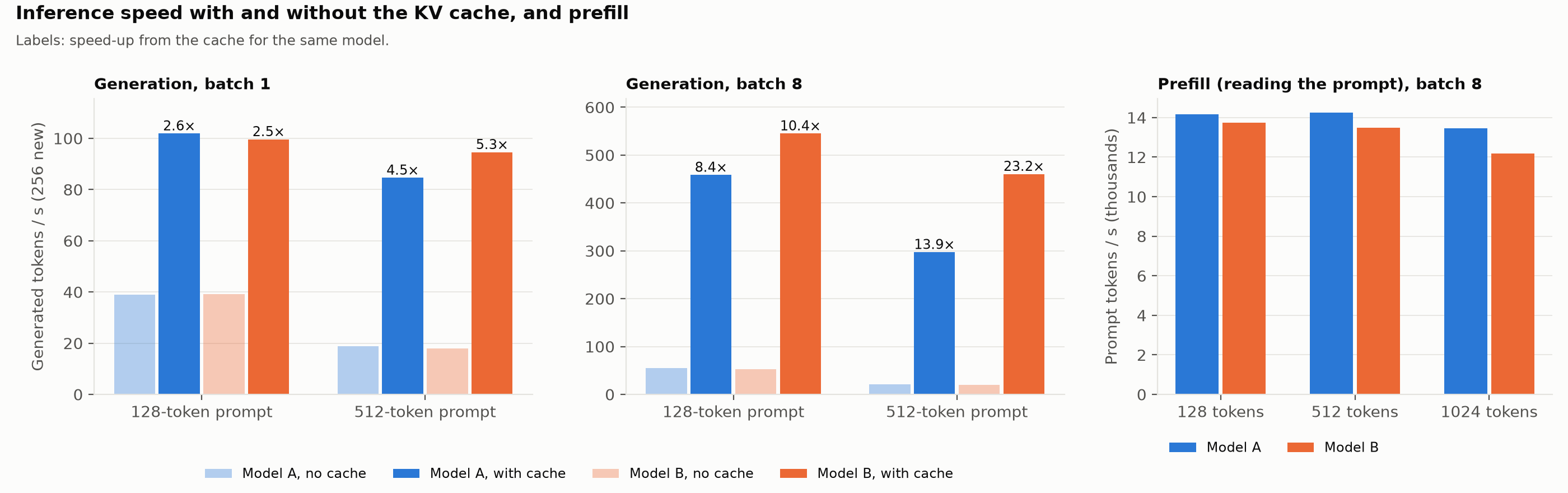
  <li>Model B is cheaper for inference: Its grouped-query attention and local windows make its KV cache 6.4x smaller, so it can serve
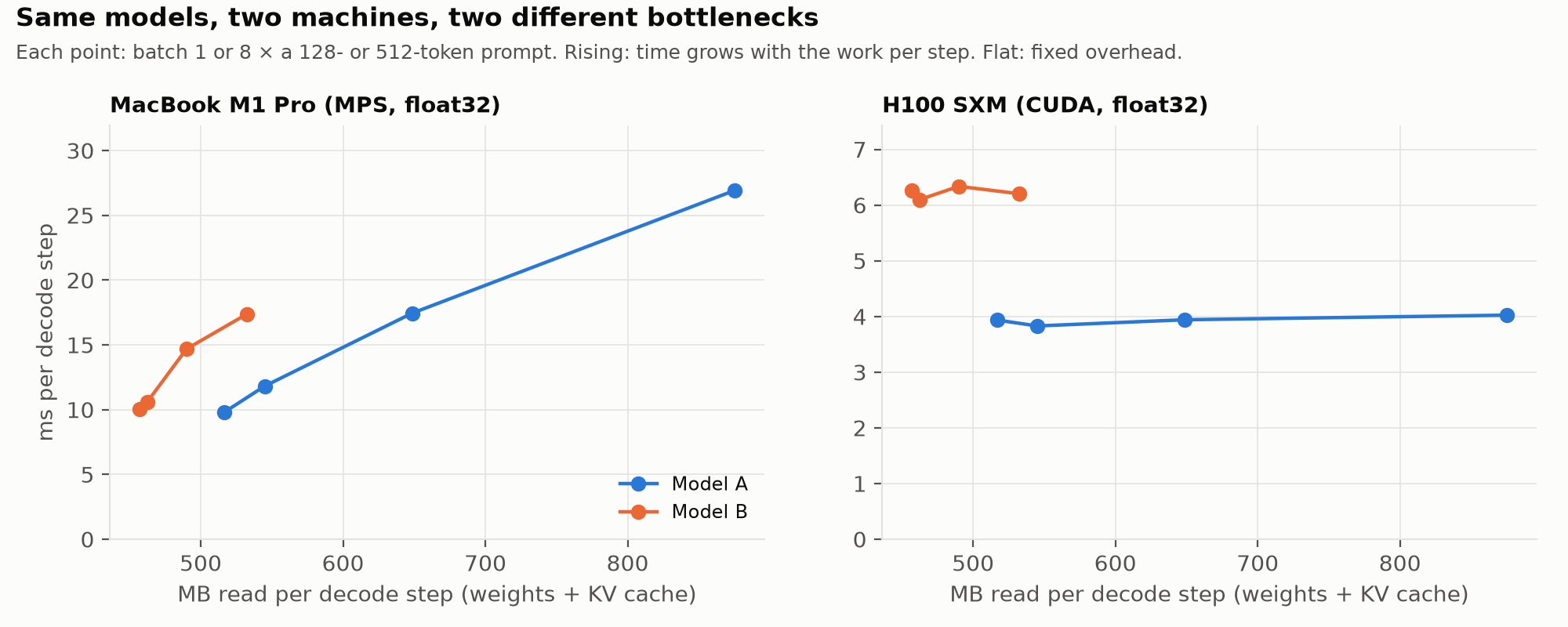
longer contexts and more sequences compared to Model A. At this model scale, whether that makes token generation faster
depends on the hardware (Part 2).</li>
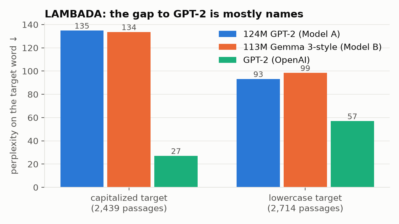
  <li>Data matters more than architecture: Against the original GPT-2 <a href="#ref-1">[1]</a>, which was trained on different data, both models gain about 8 accuracy points on science questions (ARC-Easy benchmark) and lose 8 on predicting the last word of a story passage (LAMBADA benchmark). I traced most of that loss to one capability: copying a character’s name from earlier in the story.</li>
  <li>Changing the data gives back part of that capability: Swapping half the training data for synthetic
textbooks and stories (Cosmopedia-v2) raised LAMBADA accuracy 2.3 points, at
the cost of 12.7% higher perplexity on FineWeb-Edu.</li>
</ul>

<p>The specific numbers may not hold at larger scale, but the measurement methods should.</p>

<h2 id="setup">Setup:</h2>

<h3 id="model-architecture">Model architecture</h3>

<p>Model A is GPT-2 small <a href="#ref-1">[1]</a>, exactly as <a href="https://github.com/karpathy/nanoGPT">nanoGPT</a> builds it. It has 12 layers (\(L\)), 12 attention heads, a model dimension
(\(d_{model}\), or simply \(d\)) of 768, and a 1024-token context, with
learned absolute position embeddings, full multi-head attention in every layer, a GELU MLP, and LayerNorm before each
sub-layer.</p>

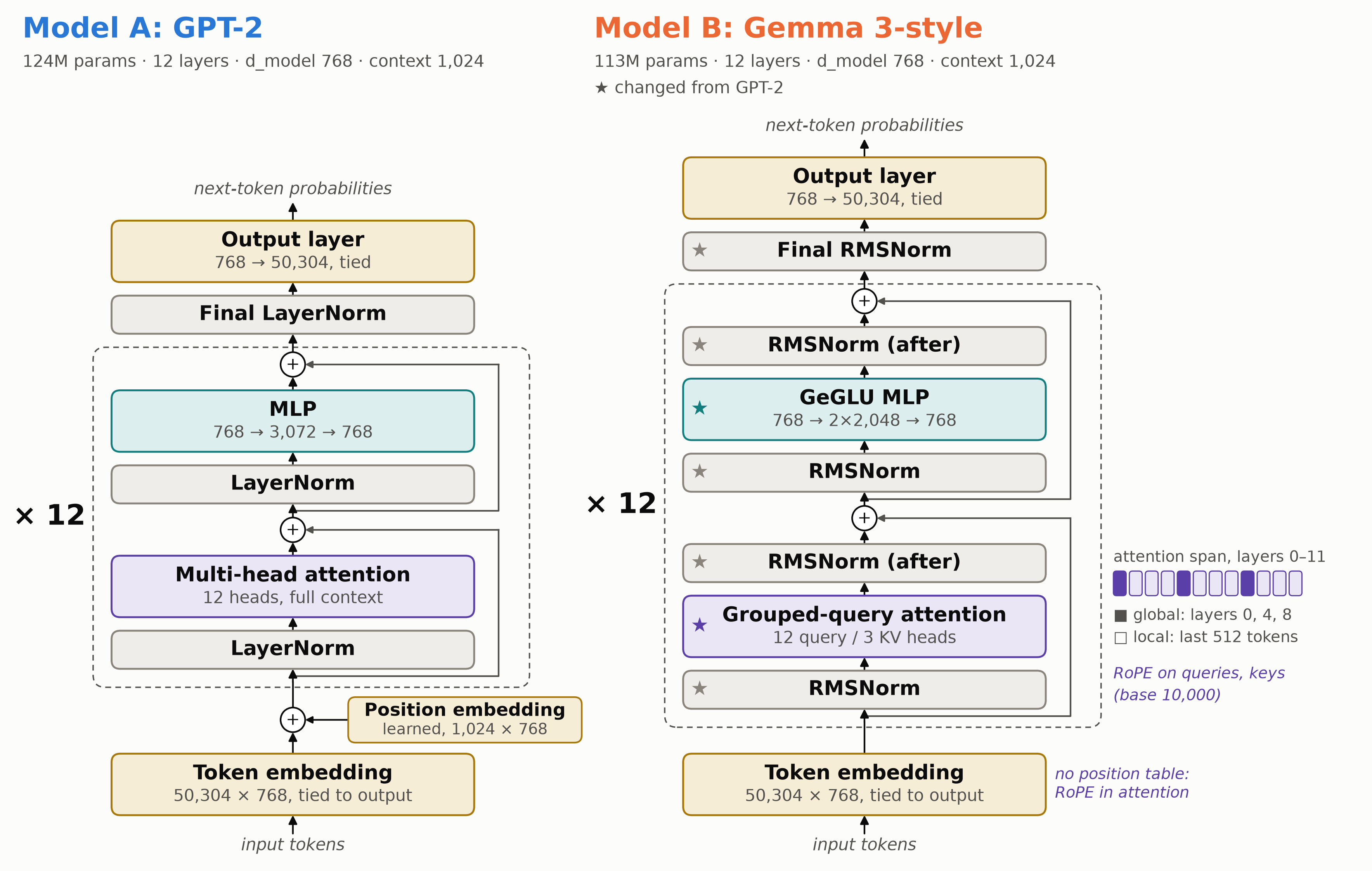
<p>Model B keeps the same skeleton (12 layers, 12 query heads, \(d = 768\), 1024 tokens) and swaps in Gemma 3-style
components. It is <strong>not an exact copy of Gemma 3</strong>: I only took the architectural changes from Gemma-3, while keeping the parameter count upper bounded to GPT-2 small.</p>

<p>What each change is meant to do, what it did in these runs, and where to read more (the inference column is measured
in Part 2):</p>

<table>
  <thead>
    <tr>
      <th>Change</th>
      <th>What it does</th>
      <th>During training</th>
      <th>At inference</th>
      <th>Deep-dive references</th>
    </tr>
  </thead>
  <tbody>
    <tr>
      <td>RoPE</td>
      <td>instead of learned positions, queries and keys are rotated by an angle so attention sees <em>relative</em> distance</td>
      <td>The only change that improved loss (−0.085 at 1.5B tokens); 0.8M fewer parameters</td>
      <td>No effect on cache size; makes context extension (YaRN) possible</td>
      <td>Su et al. 2021 <a href="#ref-3">[3]</a>; Gordić’s <a href="https://www.aleksagordic.com/blog/transformer">article</a></td>
    </tr>
    <tr>
      <td>Grouped-query attention</td>
      <td>12 query heads share 3 key/value heads (4:1 Q-KV head ratio)</td>
      <td>No measurable quality change; 8% fewer FLOPs per token; the fastest of the ablation runs below</td>
      <td>4× smaller KV cache</td>
      <td>Ainslie et al. 2023 <a href="#ref-4">[4]</a></td>
    </tr>
    <tr>
      <td>GeGLU + sandwich RMSNorm</td>
      <td>GeGLU is a gated variant of the GELU MLP. A gated MLP has three weight matrices instead of two, so its inner width is cut to 2/3 of GPT-2’s (2048 instead of \(4d\) = 3072) to keep the parameter count level. “Sandwich” norm applies RMSNorm both before and after each attention and MLP block, for smoother optimization</td>
      <td>Within noise; same FLOPs (narrower MLP); slower, from extra elementwise operations</td>
      <td>No effect</td>
      <td>Shazeer 2020 <a href="#ref-5">[5]</a>; Zhang &amp; Sennrich 2019 <a href="#ref-6">[6]</a></td>
    </tr>
    <tr>
      <td>Local/global attention</td>
      <td>3 of every 4 layers only attend to the most recent 512 tokens; every fourth layer sees the full context. Per layer, attention looks like <em>GLLLGLLLGLLL</em></td>
      <td>Within noise at a 1024-token context; slower unless the kernel skips masked blocks</td>
      <td>In 3 of 4 layers, the cache stops growing at 511 past positions</td>
      <td>Gemma 2 and 3 reports <a href="#ref-7">[7]</a>, <a href="#ref-8">[8]</a></td>
    </tr>
  </tbody>
</table>

<p>Gemma 3’s local window is 1024 tokens, which would cover
this model’s entire 1024-token context and make its local layers global, so Model B’s window is half the
context, 512 tokens. Model B also keeps one global layer in every four rather than Gemma 3’s one in six, and leaves
out Gemma 3’s QK-norm, which I didn’t test.</p>

<table>
  <thead>
    <tr>
      <th> </th>
      <th>Model A (GPT-2 recipe)</th>
      <th>Model B (Gemma 3 recipe)</th>
    </tr>
  </thead>
  <tbody>
    <tr>
      <td>Parameters</td>
      <td>124.5M</td>
      <td>113.1M</td>
    </tr>
    <tr>
      <td>Position information</td>
      <td>learned table, 1024 × 768</td>
      <td>RoPE (no parameters)</td>
    </tr>
    <tr>
      <td>Attention</td>
      <td>12 heads, all global</td>
      <td>12 query / 3 KV heads; 3 of 4 layers local (512)</td>
    </tr>
    <tr>
      <td>MLP</td>
      <td>GELU, 3072 wide</td>
      <td>GeGLU, 2,048 wide</td>
    </tr>
    <tr>
      <td>Norm</td>
      <td>LayerNorm, pre</td>
      <td>RMSNorm, pre and post</td>
    </tr>
  </tbody>
</table>

<p><img src="/assets/s1/figures/architecture.png" alt="The two architectures side by side: GPT-2 and the Gemma 3-style recipe, as trained" /></p>

<p>Model B ends up with 9% fewer parameters, and almost all of the difference is GQA’s smaller key/value projections. I
didn’t enlarge \(d\) to scale up the parameter count, because the comparison holds the shape of the transformer blocks fixed, and does not fixate the parameter total. At this size, a large share of the parameters sits in the token
embedding table: 31% of Model A’s. Google’s smallest Gemma, <a href="https://developers.googleblog.com/en/introducing-gemma-3-270m/">Gemma 3 270M</a> is more extreme, about 170M of its parameters are in the
embedding table, because its vocabulary has 256K entries, and only about 100M are in its transformer blocks. Our models
use GPT-2’s BPE tokenizer’s 50K vocabulary, so their embedding table is far smaller, and Model B’s transformer blocks (about 74M
parameters) are the same order of magnitude as Gemma 3 270M.</p>

<p>The embedding share is itself a small-model effect. With a vocabulary of \(V\) entries, the embedding table holds \(V·d\) parameters, while the \(L\) transformer blocks hold \(\sim 12·L·d^2\): \(4d^2\) in each
layer’s attention projections (Q, K, V and output) and \(8d^2\) in its MLP (up and down projections). So the table’s share falls quickly with size: 31% of GPT-2 small, 15% of GPT-2 medium, 5%
of GPT-2 XL. At 124M, whether you account for the embedding table changes the parameter count a lot but at larger scale, it barely does.</p>

<h3 id="data-and-tokenizer">Data and tokenizer</h3>

<p>Following nanoGPT’s recipe, both models train on <a href="https://huggingface.co/datasets/HuggingFaceFW/fineweb-edu">FineWeb-Edu</a> (the <code class="language-plaintext highlighter-rouge">sample-10BT</code>
subset). Hugging Face built it by scoring web pages for educational value; in their
ablations it was the strongest open web corpus for small models. Both our models use GPT-2’s BPE tokenizer (vocabulary \(50257\)). It is byte-level, so any text (emojis included as we will see in Part 2) can be encoded without
“unknown” tokens. As in nanoGPT, the embedding and output layers pad the vocabulary from 50257 up to \(V = 50304\), the next multiple of 64. Why multiple of 64? GPUs compute matrix products in fixed-size tiles, so a dimension that doesn’t divide evenly leaves a last tile that is mostly empty work. For 16-bit math, NVIDIA recommends dimensions that are multiples of 64 <a href="#ref-26">[26]</a>. Besides, The 47 extra vocabulary rows we appended are never used as target during training, so the model learns to assign near-zero probability to them.</p>

<p>The data is tokenized once, into 100M-token shards (99 training and 1 validation). Each document is
prefixed with GPT-2’s end-of-text token, <code class="language-plaintext highlighter-rouge">&lt;|endoftext|&gt;</code> (EOT), and the documents are concatenated back to back:</p>

<div class="language-plaintext highlighter-rouge"><div class="highlight"><pre class="highlight"><code>[EOT, doc 1 tokens…, EOT, doc 2 tokens…, EOT, doc 3 tokens…, …]
</code></pre></div></div>

<p>A shard is cut every 100M tokens, so a document that runs past the cut continues at the start of the next shard. The
EOT marks where one web page ends and the next begins, so the model learns not to read one into the other. Training
sequences are cut from this stream every 1024 tokens, regardless of document boundaries.</p>

<h3 id="training">Training</h3>

<p>Both models use nanoGPT’s GPT-2 recipe unchanged: AdamW optimizer with a peak learning rate of 6e-4 decaying to 6e-5 on a
cosine schedule, \(\beta_2= 0.95\), weight decay \(0.1\) and gradient clipping at \(1.0\). Training runs in bf16 with
<code class="language-plaintext highlighter-rouge">torch.compile</code> on rented H100s, with PyTorch’s Distributed Data Parallel (DDP): every GPU holds a full copy of the
model, processes its own slice of the data, and the GPUs average their gradients before each optimizer step.</p>

<p>Three numbers dictate how much data a step sees. Each GPU processes a micro-batch of \(B = 60\) sequences of \(T = 1024\)
tokens at a time. Gradients from \(G = 8\) micro-batches are accumulated before the optimizer updates the weights, and \(G\) is split across the GPUs (4 micro-batches each on 2 GPUs, 2 each on 4). So every optimizer step sees \(B·T·G = 491520\) tokens, however many GPUs share the work.</p>

<p>I didn’t tune that step size. GPT-3 <a href="#ref-2">[2]</a> trained its 125M model with batches of about 0.5M tokens, and
nanoGPT’s GPT-2 config reaches ~0.5M as 491,520 tokens (12 sequences × 1024 tokens × 40 micro-batches). Keeping that
number keeps the optimization identical to nanoGPT; only the split between \(B\) and \(G\) was chosen for the hardware, with \(B·G = 480\)
sequences fixed.</p>

<p>Both models read the shards in the same order. On each micro-batch, the \(N_{GPU}\) GPUs together read one contiguous
block of \(N_{GPU}·B·T\) tokens from the current shard, GPU \(r\) reading the \(r\)-th slice of \(B·T\) tokens, and then all
of them stride forward by \(N_{GPU}·B·T\) tokens. Over one optimizer step they cover 491520 consecutive tokens.</p>

<h2 id="the-ladder-one-change-at-a-time">The ladder: one change at a time</h2>

<h3 id="step-wise-changes-at-small-scale">Step-wise changes at small scale</h3>
<p>Architectural changes (and also hyperparameter sweeps) are cheapest to test on short runs, so the project has two stages. First, a ladder of five runs (let’s call them “rungs”) of 1.5B tokens each (~15% of the full budget), each rung adding one change to the one before; each took about 0.5 hours on 2 H100s. Then the two ends of the ladder, GPT-2 small and the full Gemma 3-style recipe, trained on the full 9.8B tokens (about 1.6 hours each on 4 H100s), with the same
data and the same hyperparameters. Each run’s settings came from one model config and a couple of environment variables, and every run logged
to my Weights &amp; Biases account.</p>

<table>
  <thead>
    <tr>
      <th>Rung</th>
      <th>Adds</th>
      <th>Parameters</th>
      <th>Val loss</th>
      <th>Step vs previous</th>
    </tr>
  </thead>
  <tbody>
    <tr>
      <td>a0</td>
      <td>nothing: GPT-2 as nanoGPT ships it</td>
      <td>124.5M</td>
      <td>3.495</td>
      <td> </td>
    </tr>
    <tr>
      <td>a1</td>
      <td>RoPE instead of learned positions</td>
      <td>123.7M</td>
      <td>3.410</td>
      <td><strong>−0.085</strong></td>
    </tr>
    <tr>
      <td>a2</td>
      <td>grouped-query attention, 4 query heads per K/V head</td>
      <td>113.1M</td>
      <td>3.431</td>
      <td>+0.021</td>
    </tr>
    <tr>
      <td>a3</td>
      <td>GeGLU MLP, RMSNorm before <em>and</em> after each sub-layer</td>
      <td>113.1M</td>
      <td>3.454</td>
      <td>+0.023</td>
    </tr>
    <tr>
      <td>a4</td>
      <td>local attention (512-token window) in 3 of every 4 layers</td>
      <td>113.1M</td>
      <td>3.455</td>
      <td>+0.001</td>
    </tr>
  </tbody>
</table>

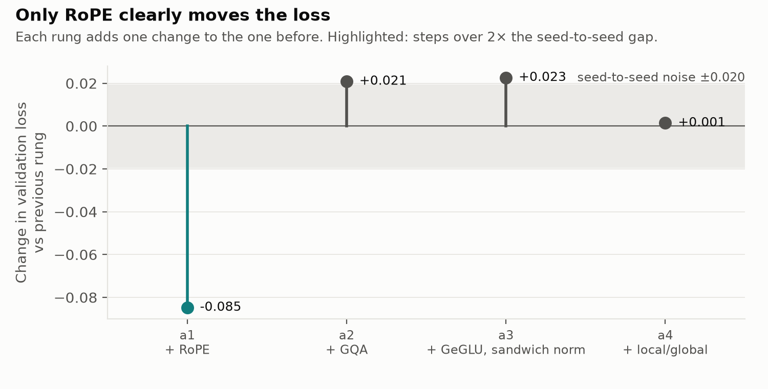
<p>Each step is the difference between two single training runs, so it carries the run-to-run noise of both. To size
that noise, I trained one rung (a4) twice with different random seeds. The two copies ended 0.020 apart; the figure draws that gap as the noise band.</p>

<p><img src="/assets/s1/ladder/figures/ladder_loss.png" alt="Each rung's step against the seed noise band" /></p>

<p>RoPE’s step is four times the seed-to-seed gap. It is the one change that makes the model
better at this scale, and it does so with <em>fewer</em> parameters, since the learned position table (0.8M parameters)
disappears. GQA and GeGLU each cost about 0.02 in val loss, right at the edge of the band. Either could be real or noise,
and it would take two or three more seeds per rung to conclude. I didn’t run those extra seeds, since the GPU hours were better spent on the full-length runs. Local attention changes nothing measurable, as expected at a 1024-token context, where a local
512-token window still sees half of all previous tokens in the full context.</p>

<h3 id="training-throughput-and-kv-cache-per-rung">Training throughput and KV cache per rung</h3>

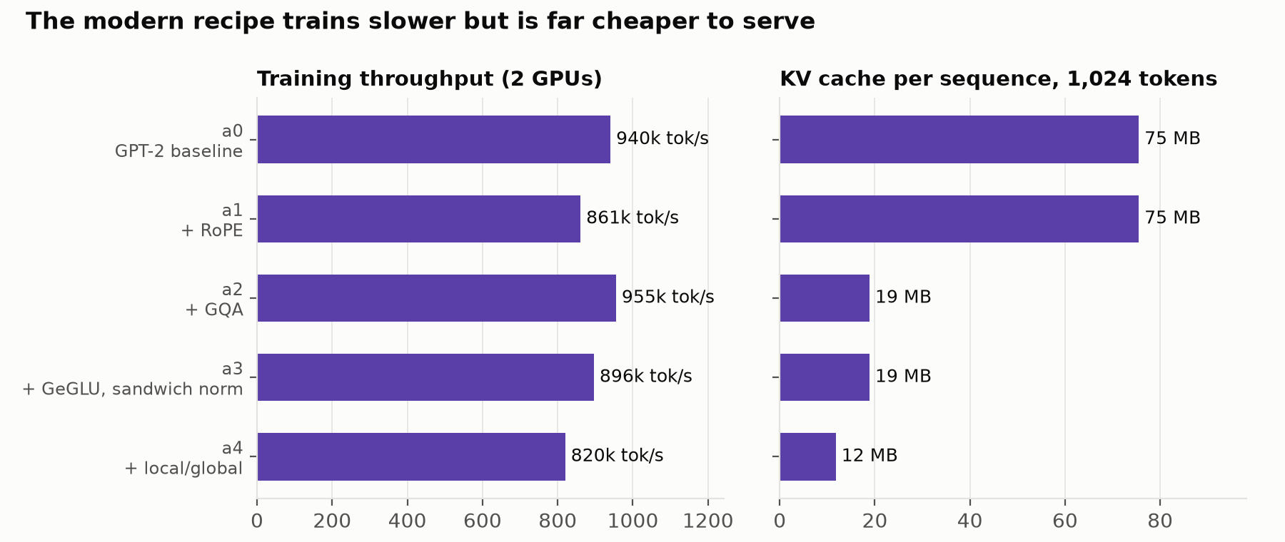
<p><img src="/assets/s1/ladder/figures/ladder_efficiency.png" alt="Training throughput and KV-cache size per rung" /></p>

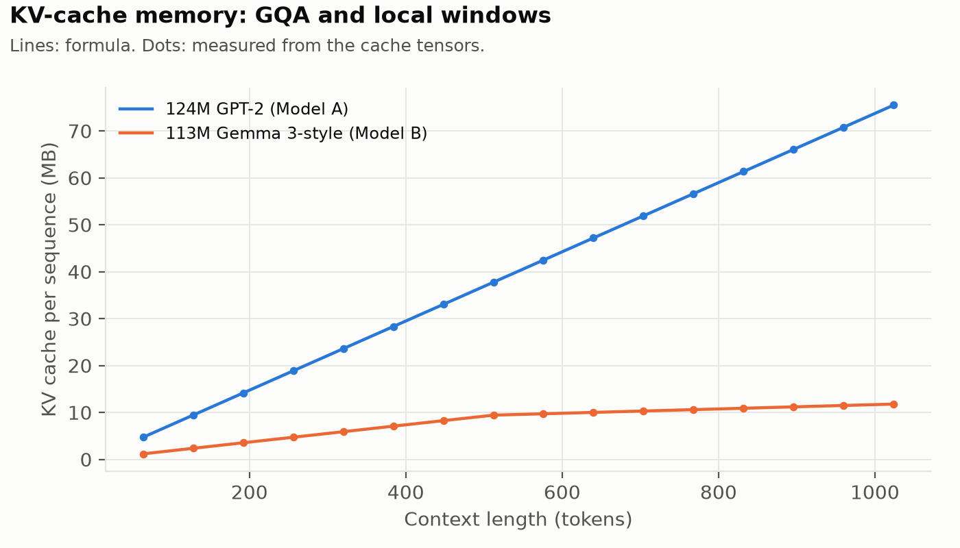
<p>The right panel shows how GQA and local attention helps at inference time. When a model generates text, it stores the keys and values of every past token (the KV cache). GQA cuts that cache by 4x, from 75 to 19 MB per 1024-token sequence, because 12 query heads now share 3 key/value heads. Local windows take it down to 12 MB (6.4x smaller than Model A), because three layers in four keep only the last 511 positions (the 512-token window includes the current token). These sizes assume float32 keys and values: for Model A, 2 (K and V) × 12 layers × 1024 tokens × 768 dimensions × 4 bytes \(\approx\) 75 MB. In bf16, the size halves.</p>

<p>The left panel shows that the Gemma 3 recipe trains <em>slower</em> at 820k tokens per second against GPT-2’s 940k.
Two rungs each cost about 8.5% extra time. One is RoPE, whose rotations add elementwise work on every query and key. The other is local
attention. Restricting attention to a window meant handing PyTorch’s scaled dot-product attention function an
explicit mask, and PyTorch can’t run its FlashAttention kernel <a href="#ref-14">[14]</a> with an arbitrary mask. It falls back to a
general-purpose kernel that scores every query-key pair, including the ones the window then throws away.
FlexAttention <a href="#ref-15">[15]</a> builds the window into a block mask instead, and skips the tiles of the attention matrix that
are fully masked. On the same two H100s, it cut rung a4’s time per optimizer step from about 590 ms to about 560 ms
(about 5% faster, MFU 33.4% → 35.2%), but didn’t close the whole gap. The ladder figure above shows the dense-mask
version but the final 9.8B-token Model B run used FlexAttention.</p>

<p>GQA, the one change that cuts training FLOPs by a meaningful amount (8%; the local windows cut another 1%), is the
fastest rung. In short, at 124M, RoPE is the change that helps quality, GQA and local windows reduce serving cost, and
GeGLU with sandwich norm can’t be told apart from noise. A general intuition about “why sandwich norms?” from literature survey <a href="#ref-27">[27]</a>: Normalizing each sublayer’s output as well as its input caps how much any one layer can add to the residual stream, which keeps activations and gradients in a steady range as the model trains .</p>

<h3 id="how-this-compares-with-published-results">How this compares with published results</h3>

<p>The papers behind these changes, at billions of parameters, report the same split between quality and cost:</p>

<ul>
  <li>The GQA paper (Ainslie et al. 2023) <a href="#ref-4">[4]</a> finds GQA close to full multi-head attention quality,
at close to multi-query attention speed.</li>
  <li>Gemma 3’s report <a href="#ref-8">[8]</a> describes its move to more local layers and shorter windows as cutting KV-cache memory with little
effect on perplexity.</li>
  <li>RoPE has become the standard position encoding in open models, including Llama, Qwen and Gemma.</li>
  <li>GLU variants are where the ladder and the literature differ: Shazeer (2020) <a href="#ref-5">[5]</a> reports lower perplexity from gated MLPs
in T5 pretraining, while here the change sits at the edge of seed noise.</li>
</ul>

<h2 id="confirming-at-our-full-98b-token-budget">Confirming at our full 9.8B token budget</h2>

<p>A change that helps at 1.5B tokens can flatten out once the model has seen more data, so I trained the two ends of the ladder on the full budget: Model A (vanilla GPT-2) and Model B (the full Gemma 3-style recipe). Each run is 20,000 steps of 491,520 tokens, or 9.83 billion FineWeb-Edu tokens: a round number of steps that stays just inside the 99 training shards (9.9B tokens), so it is a single pass with no
repeated data. That’s roughly 4x the “compute-optimal” budget the Chinchilla scaling law <a href="#ref-9">[9]</a> suggests for this model size.</p>

<p>The loss throughout is cross-entropy: the average negative natural log of the probability the model gave each correct next
token, over \(N\) tokens. Because it uses the natural log, its unit is the <em>nat</em>. Perplexity is the same quantity exponentiated, and can be interpreted as the number of tokens the model is effectively choosing between:</p>

\[\text{loss} = -\frac{1}{N}\sum_{i=1}^{N} \ln p(x_i \mid x_{&lt;i}) \qquad \text{perplexity} = e^{\text{loss}}\]
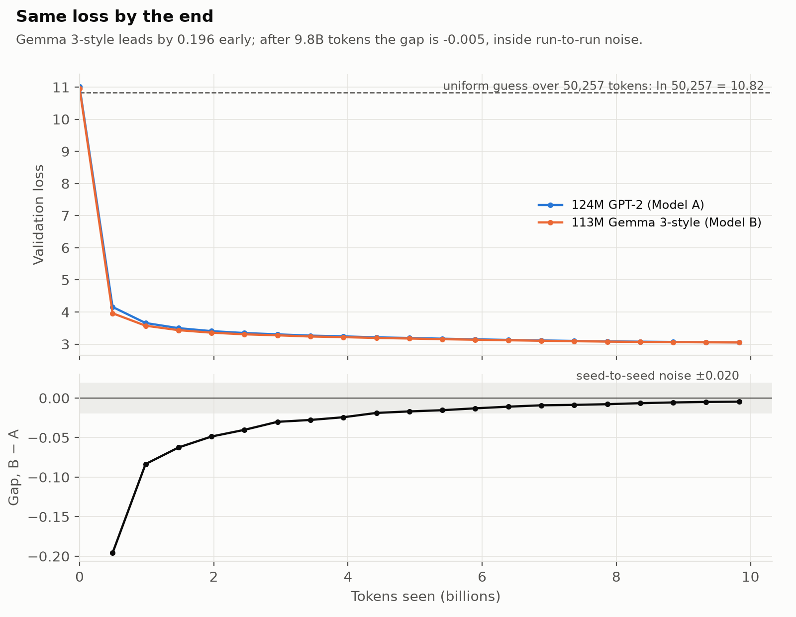
<p><img src="/assets/s1/headline_comparison/figures/loss_overlay.png" alt="Validation loss of both models over 9.8B tokens, and the gap between them" /></p>

<p>Both curves start near \(\ln (50257) ≈ 10.8\), the loss of guessing uniformly over
50257 tokens (excluding the padded vocabulary). Train and validation loss track each other the whole way, as expected when no example is seen twice. The first 0.5B tokens cut the loss by 2.75x; after that it improves slowly. The bottom panel shows the gap between the two models’ validation loss.</p>

<p>Model B pulls ahead immediately, which our ladder rungs attributes mostly to RoPE. After 0.5B tokens, B is ahead by 0.196, ten times the
seed-noise gap. Then the gap closes. By about 4.4B tokens it is inside the seed-noise band, and at the
end it is 0.005, with B at 3.0506 and A at 3.0553. That’s a tie as the gap is a quarter of the difference between two
seeds of the same model. At this size, Model B’s architecture gets to a given loss sooner but does not end lower. Whether the two endpoints separate at
larger scale is a question these runs can’t answer.</p>

<h2 id="training-on-a-budget-flops-mfu-and-what-a-run-costs">Training on a budget: FLOPs, MFU and what a run costs</h2>

<h3 id="counting-flops">Counting FLOPs</h3>

<p>The counts below are for the forward pass: what it costs to run one token through the model, which is also what
inference pays per token. Training adds a backward pass, which costs about twice the forward, so about 3x in total.</p>

<p>Almost all of a transformer’s arithmetic is matrix multiplication. Multiplying a token’s \(m\)-dimensional vector by an \(m × n\) weight matrix costs ~\(2mn\) FLOPs: one multiply and one add per weight. Applying this to each piece of a
layer gives <strong>266M</strong> FLOPs per token for Model A and <strong>241.2M</strong> for Model B; the full
derivation is in the appendix (<a href="#counting-the-flops">Counting the FLOPs</a>).</p>

<p>The count leaves out everything that isn’t a matrix multiplication: biases, normalization, activations, softmax and
masking, RoPE’s rotations, residual additions, the embedding lookup and the loss. By a rough count they add up to under 1% of
the FLOPs, but they take far more than 1% of the time: each one reads and writes whole tensors from memory while
doing very little arithmetic, as <a href="#how-well-the-gpus-were-used">How well the GPUs were used</a> shows below.</p>

<p>With \(d\) being the
model dimension, \(T\) the context length and \(k̄\) the average number of keys a query attends to, four insights to notice:</p>

<ul>
  <li>GeGLU costs exactly what GELU costs: With the hidden width trimmed to \(8d/3\), both MLPs land at \(16d^2\) FLOPs, so any
difference between rungs a2 and a3 can’t be a compute difference.</li>
  <li>GQA’s saving is in the Q, K, V projections: which drop from \(6d^2\) (A) to \(3d^2\) (B) per layer. That is 21.2M FLOPs per token, 8 of the 9 percentage points
Model B saves over Model A. The local windows supply the last point (3.5M) by shortening \(k̄\) in nine layers.</li>
  <li>Attention is the only term that grows with context length: Per layer, the attention scores cost \(2d(T + 1)\)
against \(24d^2\) for the weight matrices, a ratio of \((T + 1)/(12d)\). At \(T = 1024\) and \(d = 768\) that’s 11%, so
attention is about \(10\%\) of each layer’s FLOPs (about \(7\%\) of the whole forward pass, once the output layer is
counted). At this size and context, local windows don’t save many FLOPs; their payoff is in the KV cache.</li>
  <li>Without the attention term, the forward pass is 2 FLOPs per weight: and
training (the forward pass plus a backward pass costing about 2x the forward) is \(2 + 4 = 6\) FLOPs per weight:
the well-known \(6N\). The attention term adds \(6·L·d·(T + 1)\) on top.</li>
</ul>

<h3 id="where-the-flops-go">Where the FLOPs go</h3>

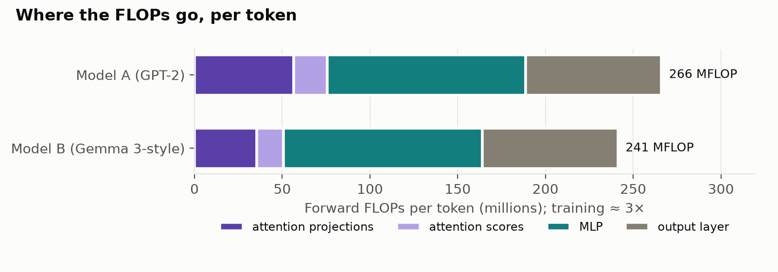
<p><img src="/assets/s1/efficiency/figures/flops.png" alt="Forward FLOPs per token, by component" /></p>

<p>At this model scale, the output layer is almost 1/3 of the total compute: projecting onto the
50,304-entry padded vocabulary costs 2/3 as much as the whole MLP stack.
Training costs about 3x the forward pass: 798 MFLOP per token for Model A and 724 for Model B. Over 9.83B tokens, that’s \(7.8 × 10^{18}\) and \(7.1 × 10^{18}\) FLOPs. The plain \(6N\) rule comes within 7% of these numbers; the
difference is the attention term.</p>

<h3 id="how-well-the-gpus-were-used">How well the GPUs were used</h3>

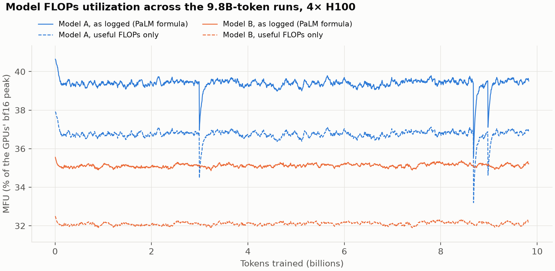
<p>Model FLOPs utilization (MFU) is the FLOPs a run actually achieves per second, divided by what the hardware can do
at peak. For an H100 SXM in bf16, the peak is 989 TFLOP/s: <a href="https://www.nvidia.com/en-us/data-center/h100/">NVIDIA’s spec sheet</a>
lists 1,979 TFLOP/s “with sparsity”, and dense matrix multiplication gets half that.</p>

<table>
  <thead>
    <tr>
      <th>Headline runs, 4× H100</th>
      <th>Model A</th>
      <th>Model B</th>
    </tr>
  </thead>
  <tbody>
    <tr>
      <td>Throughput</td>
      <td>1.82M tokens/s</td>
      <td>1.76M tokens/s</td>
    </tr>
    <tr>
      <td>MFU, as the training script logs it (PaLM formula)</td>
      <td>39.4%</td>
      <td>35.1%</td>
    </tr>
    <tr>
      <td>MFU, counting only useful FLOPs</td>
      <td>36.8%</td>
      <td>32.1%</td>
    </tr>
    <tr>
      <td>GPU-hours for 9.83B tokens</td>
      <td>6.0</td>
      <td>6.2</td>
    </tr>
  </tbody>
</table>

<p>The training script, following nanoGPT, logs MFU with the PaLM paper’s <a href="#ref-11">[11]</a> formula. It counts \(12·L·d·T\) FLOPs for attention, which charges every token for attending to
the whole context. Counting only the attention a causal model actually computes (and, for Model B’s local layers, only the keys inside the window) gives the “useful FLOPs” row, a few points
lower. B loses more, because the PaLM formula also charges its local
layers for keys they skip. The gap is small at 1024 tokens and grows with context; <a href="https://shinibali.github.io/gpt2-to-gemma-part-2/">Part 2</a> works out by how much.</p>

<p><img src="/assets/s1/efficiency/figures/mfu.png" alt="MFU across the two 9.8B-token runs, as logged and counting useful FLOPs only" /></p>

<p>The training script logs a running average of MFU, in which each new step’s reading counts for 10%, and it leaves
out the steps that also ran an evaluation or saved a checkpoint. So the remaining dips are real stretches where steps
ran slower, for reasons the logs don’t record. Model B does 9% fewer FLOPs per token, yet it runs 4% slower, so it spends more time on work that isn’t matrix multiplication:</p>
<ul>
  <li>two extra normalizations per block;</li>
  <li>the gating multiply in GeGLU;</li>
  <li>the rotations in RoPE;</li>
  <li>the attention kernel’s handling of the local windows.</li>
</ul>

<p>Each of these is cheap in FLOPs but has to read and write whole activation tensors from memory. In <a href="https://horace.io/brrr_intro.html">Horace He’s terms</a>,
they’re memory-bandwidth-bound, not compute-bound, which is why fewer FLOPs did not mean a faster run.</p>

<h3 id="how-the-balance-shifts-as-models-and-contexts-grow">How the balance shifts as models and contexts grow</h3>

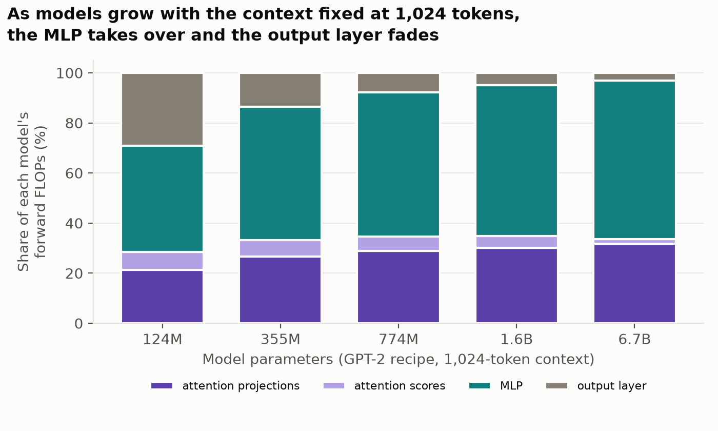
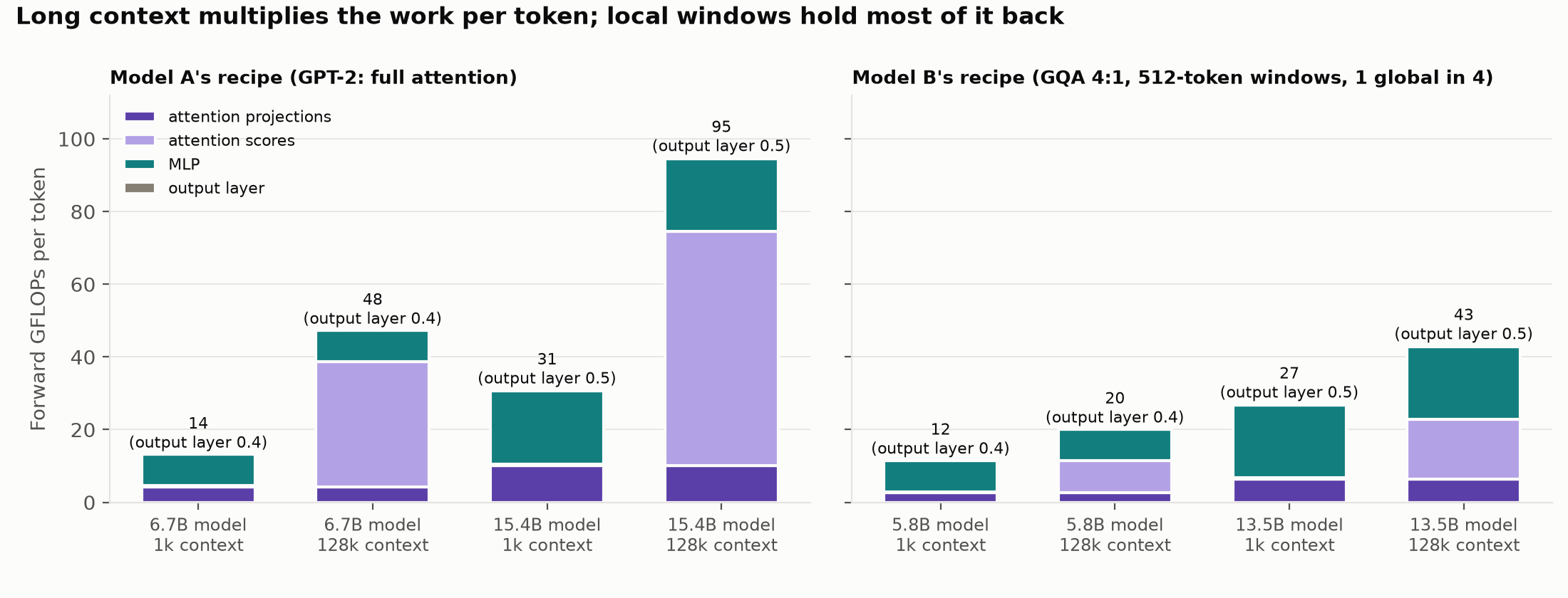
<p>The equations in <a href="#counting-the-flops">Counting the FLOPs</a> show how each component’s share of the FLOPs moves with scale. The MLP and attention
projections grow with \(d^2·L\), the output layer with \(d·V\), and the attention scores
with \(d·T·L\), the only term that depends on context. The figure below holds the context at 1024 tokens and follows the GPT-2 recipe from 124M up through GPT-2 XL (1.6B) to a 6.7B model: the output layer shrinks from 29% of the forward pass to 5% and then about 3%, and the MLP becomes the majority.</p>

<p><img src="/assets/s1/efficiency/figures/flops_by_size.png" alt="Each component's share of a model's forward FLOPs, from 124M to 6.7B parameters" /></p>

<p>Two crossovers follow from the same terms. Attention overtakes the MLP at \(T ≈ 8d\), about 6,000 tokens at our \(d\) of 768; <a href="https://shinibali.github.io/gpt2-to-gemma-part-2/">Part 2</a> follows that term to long contexts. The crossover that matters at this
size is the output layer: its \(2dV\) FLOPs outweigh all the MLPs together (\(16d^2·L\)) while \(d·L &lt; V/8\). With the padded 50304-entry
vocabulary, \(V/8 ≈ 6288\). Our models sit at \(d·L = 9216\), just past the crossover, which is why the output layer costs
2/3 as much as the MLPs here. A model with Gemma 3’s 262,144-entry vocabulary needs \(d·L\) above about 33,000 before
its MLPs outweigh its output layer.</p>

<h3 id="getting-the-gpus-busy-in-the-first-place">Getting the GPUs busy in the first place</h3>

<p>The first runs on the H100s reached an MFU of only about 25%, with a micro-batch \(B\) of 12 sequences per GPU. A
124M model is small enough that, at 12 sequences per GPU, a large share of every step goes to fixed
overheads: launching kernels, moving small tensors, synchronizing. Raising the micro-batch to 60 sequences, and
reducing gradient accumulation to keep each optimizer step at 491,520 tokens, took MFU up to 41%. The optimizer update is mathematically identical, since
every step still sees the same tokens. Beyond 60 sequences the gain flattened out while
memory kept climbing. And because the \(G\) accumulated micro-batches are split across the GPUs, moving from 2 to 4 GPUs sped training up 1.94x with identical optimizer steps.</p>

<p>The training data never sits in GPU memory. The 100 tokenized shards (100M tokens × 2 bytes each) take 20 GB of disk.
They live in our <a href="https://huggingface.co/CuriosLM">CuriosLM Hugging Face org</a>, each pod downloads them in about a minute, and the data loader keeps only the current
200 MB shard in CPU memory. For comparison, a 15T-token corpus is 30–60 TB
once tokenized (2 to 4 bytes per token) which is too much to copy onto every machine, so larger runs typically streams training tokens from shared cloud storage.</p>

<h3 id="how-large-a-model-fits-on-one-gpu">How large a model fits on one GPU</h3>

<p>Each GPU’s memory (80 GB of HBM on an H100) holds two main things: the <strong>model state</strong>, which grows with the parameter count \(N ≈ 12·L·d^2 + V·d\), and the <strong>activations</strong> saved for the backward pass, which grow with the micro-batch of \(B\)
sequences of \(T\) tokens. The table gives the standard estimate for each, next to Model A’s measured peak memory:</p>

<table>
  <thead>
    <tr>
      <th>Per GPU</th>
      <th>Bytes</th>
      <th>Model A, \(B = 60\), \(T = 1024\)</th>
    </tr>
  </thead>
  <tbody>
    <tr>
      <td>Model state: bf16 weights and gradients, float32 master weights, AdamW’s two moments <a href="#ref-10">[10]</a></td>
      <td>\(16N\)</td>
      <td>2.0 GB</td>
    </tr>
    <tr>
      <td>Activations in the transformer blocks <a href="#ref-25">[25]</a> (without the \(T × T\) attention scores, which FlashAttention never stores)</td>
      <td>\(34·B·T·L·d\)</td>
      <td>19.3 GB</td>
    </tr>
    <tr>
      <td>Activations of the output layer: float32 logits for the loss (4 bytes each <a href="#ref-25">[25]</a>) plus the bf16 logits the layer outputs (2 bytes)</td>
      <td>\(6·B·T·V\)</td>
      <td>18.5 GB</td>
    </tr>
    <tr>
      <td>Estimated</td>
      <td> </td>
      <td>39.8 GB</td>
    </tr>
    <tr>
      <td>Measured peak</td>
      <td> </td>
      <td>41.4 GB</td>
    </tr>
  </tbody>
</table>

<p>At this size, the output layer’s activations are as large as all twelve transformer blocks’, the same small-model effect as in
the FLOPs. Since the blocks hold \(N ≈ 12·L·d^2\)
parameters, their activations \(34·B·T·L·d\) equal \(17N · B·T/(6d)\). Rounding the 17 down to 16 (a 6% error) puts both terms in the same form:</p>

\[\text{training memory } M ≈ 16N\left(1 + \frac{B·T}{6d}\right) + 6·B·T·V\]

<p>The activations equal the model state once a micro-batch holds about \(6d\)
tokens, so small models
are limited by activations and large ones by their state. The activations are the flexible part: a smaller micro-batch \(B\), made up with more gradient accumulation,
keeps the same 491,520-token optimizer step, and activation checkpointing recomputes activations instead of storing
them. The model state can’t shrink, so it sets the ceiling. Solved for \(N\), the equation gives the largest model a GPU with memory \(M\) can train. With the smallest micro-batch, \(B = 1\) sequence of \(T = 1024\) tokens, and a width typical of 3–5B-parameter models (\(d ≈ 3000\)), \(B·T/(6d) ≈ 0.06\) and
the output layer’s \(6·B·T·V\) is only 0.3 GB, so for an 80 GB H100:</p>

\[N_{max} ≈ \frac{M - 6·B·T·V}{16\left(1 + \frac{B·T}{6d}\right)} ≈ \frac{80\text{ GB} - 0.3\text{ GB}}{16 × 1.06} ≈ 4.7\text{B}\]

<p>Leaving a few GB for the CUDA context and workspace, which the equation doesn’t
count, brings it to about 4.5B. Larger models have to be split across GPUs: ZeRO <a href="#ref-10">[10]</a> (or PyTorch’s FSDP) shards the optimizer state, gradients and weights across the data-parallel GPUs; tensor parallelism splits each layer’s weight matrices across GPUs (Megatron-LM <a href="#ref-12">[12]</a>); and pipeline parallelism places different layers on different GPUs.</p>

<h2 id="interlude-the-step-320-spike">Interlude: the step-320 spike</h2>

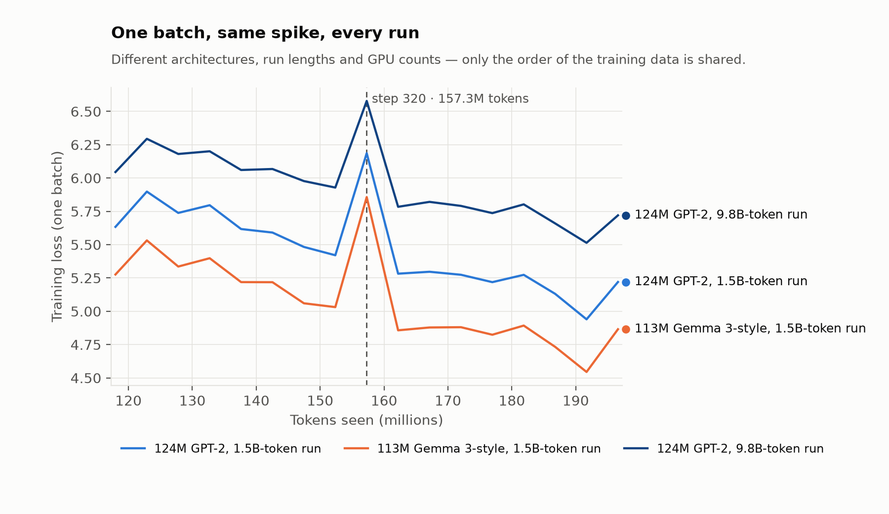
<p>While monitoring the first ladder runs, I saw a sharp spike in training loss at step 320. Loss on a single batch is noisy and spikes happen, but this one appeared at the same step in every run: both
architectures, short runs and long ones, on 2 GPUs and on 4. The only thing these runs share is the order of the
training data, so the likely cause was the data itself.</p>

<p><img src="/assets/s1/step320_spike/figures/loss_spike.png" alt="The training loss of three different runs around step 320" /></p>

<p>Because the data loader is deterministic, the batch can be replayed exactly. I rebuilt the data loader with the run’s
settings, stepped it forward to the micro-batch logged at step 320, and scored each of its 60 sequences. One
sequence stands far above the rest, with a mean loss of 5.06 against a batch median of 3.83.</p>

<p>It’s an encyclopedia-style educational page, but with
some words rewritten by a <a href="https://stackoverflow.com/beta/challenges/79640866/challenge-1-implement-a-text-to-baby-talk-translator-completed">“baby talk” text converter</a>: <em>“a totaw of”, “bewow de age of 18 years”, “broders and cwose rewatives”,
“de medod used”.</em></p>

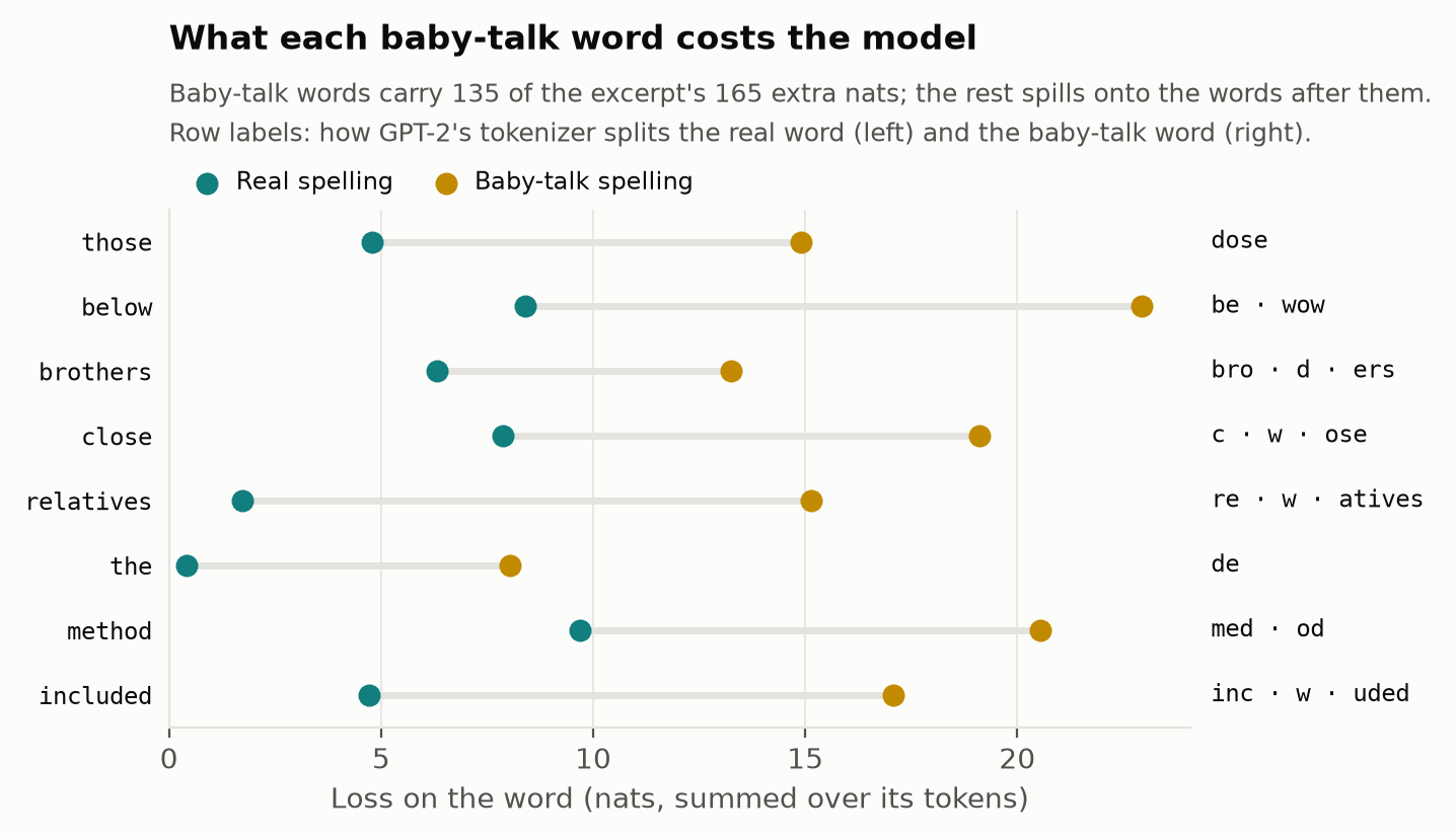
<p>The converter swaps <em>l</em> for <em>w</em> and <em>th</em> for <em>d</em> (and, more rarely, a word-final <em>th</em> for <em>f</em> and <em>qu</em> for <em>qw</em>). For the model it’s close to a
different language, and the tokenizer is where it breaks. <code class="language-plaintext highlighter-rouge">close</code> is one token, but <code class="language-plaintext highlighter-rouge">cwose</code> is
three (<code class="language-plaintext highlighter-rouge">c·w·ose</code>), each of them rare in that position. Other words turn into different words: <code class="language-plaintext highlighter-rouge">the</code> becomes ` de`, a
perfectly common token that means something else entirely, so the model has to predict a real word in the wrong place.</p>

<p><img src="/assets/s1/step320_spike/figures/word_losses.png" alt="Loss on each mangled word, real spelling vs baby talk" /></p>

<p>Comparing the page with a cleaned-up copy shows where the extra loss lives. In the excerpt shown in the figure, 11 mangled words
account for 135 of its 165 extra nats. The other 30 spill onto the words after them: once the model has seen
“bewow de”, even an ordinary “age” becomes harder to predict.</p>

<p>The cleaned copy came from a model trained in this study: the 1.5B-token checkpoint of ladder rung a4. For every word
containing a <em>w</em>, <em>d</em>, <em>qw</em> or word-final <em>f</em>, I generated every spelling the converter’s rules could have mangled
into it (each <em>w</em> may be a real <em>w</em> or an <em>l</em>, each <em>d</em> a real <em>d</em> or a <em>th</em>, and so on), and let the checkpoint pick
the one it finds most likely after the already-corrected text before it. That fixed 196 words
across the page, with one miss: a foreign word with a genuine <em>d</em> came out with a <em>th</em>, because the model had no way
to know the <em>d</em> was real.</p>

<p>Pages like this are in every web corpus, and this one did no lasting damage. The loss is back to normal on the next step, because the page is one of 60 sequences in the logged micro-batch (which is why the spike is visible) but
only one of 480 in the optimizer step. In GPT-3’s <a href="#ref-2">[2]</a> largest batch of about 3.2M tokens, it would be one in about 3,000.
Spikes in large runs therefore tend to come from the optimization itself rather than from a single bad document, and
they are harder to recover from. The PaLM paper <a href="#ref-11">[11]</a> reports about 20 spikes while training its 540B model. Its fix was to
restart from a checkpoint roughly 100 steps before each spike and skip the 200–500 data batches around it. That only
works if you can pinpoint exactly which batches those were, which is what a deterministic data loader provides, and it is also what made this diagnosis quick.</p>

<h2 id="evaluation-a-tie-on-every-benchmark">Evaluation: a tie on every benchmark</h2>

<p>Validation loss says the two models are the same. But loss is an average over every token, and two models can reach the same
average by being good at different things. So I evaluated both on a set of standard benchmarks, with OpenAI’s original GPT-2 (124M) checkpoint <a href="#ref-1">[1]</a>
(<a href="https://huggingface.co/openai-community/gpt2"><code class="language-plaintext highlighter-rouge">openai-community/gpt2</code></a> on Hugging Face) alongside as a reference, called “stock GPT-2” from
here on. All three go through the same harness, <a href="https://github.com/EleutherAI/lm-evaluation-harness">lm-evaluation-harness</a>,
connected to the models through a small custom adapter.</p>

<h3 id="choosing-benchmarks-for-a-124m-model">Choosing benchmarks for a 124M model</h3>

<p>A benchmark is only useful if the model scores clearly above chance and below the ceiling. Otherwise every
model lands on the same number and the comparison says nothing. Of the benchmarks commonly used for small models, four measures give a usable signal at this size:</p>

<ul>
  <li>HellaSwag <a href="#ref-19">[19]</a>: pick the sensible ending to an everyday scenario from 4 options. It’s the standard yardstick for small models: GPT-2-sized models score around 30%, against 25% for random guessing. Each ending is scored by its average log-probability per character, so a long ending isn’t penalized just for being long (lm-eval’s <code class="language-plaintext highlighter-rouge">acc_norm</code>).</li>
  <li>ARC-Easy <a href="#ref-20">[20]</a>: grade-school science questions. These are knowledge-heavy, so this is where training data should show.</li>
  <li>LAMBADA <a href="#ref-21">[21]</a>: predict the last word of a passage, where the word can only be guessed from the wider passage. It is the closest of the four to a test of long-range context, which is where the two models’ position schemes differ.</li>
  <li>Perplexity on held-out text from FineWeb-Edu (the training distribution) and Cosmopedia-v2 (synthetic textbooks). With no question-answer format, it tests how well each model predicts real text, and it is the least noisy number available.</li>
</ul>

<p>MMLU is left out because models this size sit at chance (25%), so it can’t tell two of them apart.</p>

<h3 id="results">Results</h3>

<p>Stock GPT-2 was trained on different data (WebText), so it is here for reference.</p>

<table>
  <thead>
    <tr>
      <th>Accuracy in %</th>
      <th>HellaSwag</th>
      <th>ARC-Easy</th>
      <th>LAMBADA</th>
    </tr>
  </thead>
  <tbody>
    <tr>
      <td>Model A (GPT-2 recipe)</td>
      <td>32.4</td>
      <td><strong>52.4</strong></td>
      <td>24.2</td>
    </tr>
    <tr>
      <td>Model B (Gemma recipe)</td>
      <td><strong>32.5</strong></td>
      <td>51.9</td>
      <td>24.5</td>
    </tr>
    <tr>
      <td>A vs B: p (paired)¹</td>
      <td>0.84</td>
      <td>0.63</td>
      <td>0.57</td>
    </tr>
    <tr>
      <td><em>Stock GPT-2 124M</em></td>
      <td><em>31.1</em></td>
      <td><em>43.8</em></td>
      <td><strong><em>32.5</em></strong></td>
    </tr>
  </tbody>
</table>

<table>
  <thead>
    <tr>
      <th>Held-out perplexity</th>
      <th>FineWeb-Edu</th>
      <th>Cosmopedia-v2</th>
    </tr>
  </thead>
  <tbody>
    <tr>
      <td>Model A</td>
      <td>21.89</td>
      <td>20.31</td>
    </tr>
    <tr>
      <td>Model B</td>
      <td>21.80</td>
      <td>20.49</td>
    </tr>
    <tr>
      <td>B − A, 95% CI¹</td>
      <td>[−0.12, −0.06]</td>
      <td>[+0.15, +0.22]</td>
    </tr>
    <tr>
      <td><em>Stock GPT-2 124M</em></td>
      <td><em>26.40</em></td>
      <td><em>20.54</em></td>
    </tr>
  </tbody>
</table>

<p>¹(A vs B is paired, since both models answer the same questions. Accuracies use McNemar’s test on per-question
correctness (McNemar, 1947) <a href="#ref-23">[23]</a>. Perplexities use a bootstrap over documents (Efron, 1979) <a href="#ref-24">[24]</a>, 10,000 resamples, because
tokens within a document aren’t independent. Both follow <a href="https://arxiv.org/abs/2411.00640">Miller (2024), <em>Adding Error Bars to Evals</em></a> <a href="#ref-22">[22]</a>.
Run-to-run (seed) noise is measured separately, from two seeds of one ladder rung.)</p>

<p><strong>None of the benchmark gaps between A and B is significant.</strong> The p-value in the table answers one question: if the
two models were equally good, how often would a gap at least this large show up just from which questions happen to be
in the test? On HellaSwag, A and B gave different answers on 841 of the 10,042 questions; A got 417 of those right and
B got 424. If each of those disagreements were a fair coin flip, a split at least this uneven would happen 84% of the
time (p = 0.84), so chance explains it easily. The usual bar for calling a difference real is p &lt; 0.05.</p>

<p>On perplexity, B is 0.09 better on FineWeb-Edu and 0.18 worse on Cosmopedia-v2. The 95% confidence interval (CI) is
the range the B − A gap would likely fall in if the test documents were resampled, and both intervals exclude zero. That makes both differences real <em>for these two checkpoints</em>, but only in the
sense that a different sample of test documents wouldn’t change them. Retraining either model with a different
random seed moves its loss by about 0.02, roughly 0.4 perplexity, which is two to four times larger than either
gap. Each checkpoint wins on one set and loses on the other.</p>

<p>The stock GPT-2 row also checks the harness: an independent lm-eval run of the same checkpoint,
published on <a href="https://huggingface.co/amd/AMD-Llama-135m">AMD’s model card for AMD-Llama-135m</a>, matches it to within
0.001 on ARC-Easy, HellaSwag and LAMBADA. Against that row, both of our models are 8 points better on ARC-Easy and 8 points worse on LAMBADA.</p>

<h2 id="data-shapes-capability-more-than-architecture">Data shapes capability more than architecture</h2>

<p>Changing the architecture did not move any benchmark significantly. Stock GPT-2 shows what changing the data does: it has the
same size and architecture as Model A but different training data. Stock GPT-2 was trained on WebText, pages linked from Reddit (2019); Models A and B
on FineWeb-Edu, web pages scored for educational value (2024).</p>

<p>Against GPT-2, both models gain on some tasks and lose on others, by large margins and in the same direction:</p>

<table>
  <thead>
    <tr>
      <th>vs stock GPT-2</th>
      <th>Model A</th>
      <th>Model B</th>
    </tr>
  </thead>
  <tbody>
    <tr>
      <td>ARC-Easy (grade-school science)</td>
      <td><strong>+8.6 pt</strong></td>
      <td>+8.1 pt</td>
    </tr>
    <tr>
      <td>HellaSwag (everyday scenarios)</td>
      <td>+1.3 pt</td>
      <td>+1.3 pt</td>
    </tr>
    <tr>
      <td>LAMBADA accuracy (last word of a story)</td>
      <td><strong>−8.2 pt</strong></td>
      <td>−7.9 pt</td>
    </tr>
  </tbody>
</table>

<p>The ARC-Easy gain is what the FineWeb-Edu authors <a href="#ref-16">[16]</a> report: filtering the web for educational content gives
<a href="https://arxiv.org/abs/2406.17557">“dramatically better performance on knowledge- and reasoning-intensive benchmarks like MMLU and
ARC”</a>.</p>

<h3 id="where-the-lambada-points-went">Where the LAMBADA points went</h3>

<p>The LAMBADA drop is a loss of a <em>capability</em> rather than of knowledge. LAMBADA passages come
from novels, and the target is the last word of the passage. The passages where GPT-2 beats Model A by the
widest margin all follow the same pattern:</p>

<blockquote>
  <p>“…He passed the glasses to Bobby who had a look. “That looks like your boy the tow truck driver, doesn’t it <strong>Bobby</strong>”</p>

  <p>“…she shifted her gaze to Gabe. “You know this through fabled stories, don’t you <strong>Gabe</strong>”</p>
</blockquote>

<p>The answer is a character’s name, mentioned earlier in the passage, so the model only has to copy it. GPT-2 usually does; our models mostly don’t.
Splitting all 5,153 passages by whether the target word is capitalized (almost always a
name) makes the pattern measurable:</p>

<p><img src="/assets/s1/headline_comparison/figures/lambada_targets.png" alt="LAMBADA perplexity by target type" /></p>

<table>
  <thead>
    <tr>
      <th>Perplexity on the target</th>
      <th>Capitalized (2,439)</th>
      <th>Lowercase (2,714)</th>
    </tr>
  </thead>
  <tbody>
    <tr>
      <td>Model A</td>
      <td>134.9</td>
      <td>93.3</td>
    </tr>
    <tr>
      <td>Model B</td>
      <td>133.7</td>
      <td>98.5</td>
    </tr>
    <tr>
      <td>GPT-2</td>
      <td>27.1</td>
      <td>57.0</td>
    </tr>
    <tr>
      <td>GPT-2’s advantage over A</td>
      <td><strong>5.0×</strong></td>
      <td>1.6×</td>
    </tr>
  </tbody>
</table>

<p>For GPT-2, names are <em>easier</em> targets than ordinary words; for our models they’re the hardest. The
architecture can’t explain that, since Model A and GPT-2 are architecturally identical, so the likely explanation is
the data. Dialogue that addresses characters by name is common in fiction, and WebText contains a lot of
fiction, because Reddit links to stories.
FineWeb-Edu filters most of it out, since fiction scores low on educational value, so our models rarely saw a name copied out of dialogue during training.</p>

<p>The mechanism for copying from context, induction heads, appears even in very small transformers
(Olsson et al., 2022) <a href="#ref-13">[13]</a>. So a bigger model trained on the same filtered data would have more capacity but no more
practice, and there’s no reason to expect scale alone to close this gap. Changing the data might.</p>

<h2 id="a-5050-data-mix">A 50:50 data mix</h2>

<p>To test that, the next run changes only the data. Model B’s architecture
and token budget stay fixed; the training data becomes half FineWeb-Edu, half
<a href="https://huggingface.co/datasets/HuggingFaceTB/smollm-corpus">Cosmopedia-v2</a>, a corpus of synthetic textbooks and
stories generated by a larger model. Hugging Face’s SmolLM2 models <a href="#ref-17">[17]</a> mix it
into their own pretraining data.</p>

<p>Mixing two datasets needs a sampling rule. The common one is random
sampling, where each batch picks a source with probability 0.5. That’s 50:50 on average, but any particular step can
be lopsided, and replaying the exact same order after a restart means saving the random generator’s state. This run
uses a deterministic rule instead, the one Megatron-LM <a href="#ref-12">[12]</a> uses to blend datasets: each micro-batch goes to whichever
dataset is furthest below its target share so far. With two datasets at 50:50 that simply alternates, but the same
rule handles any weights (90:10, three datasets, etc.) and never drifts from them by more than one micro-batch. A restart only needs to know how many micro-batches each dataset has contributed.</p>

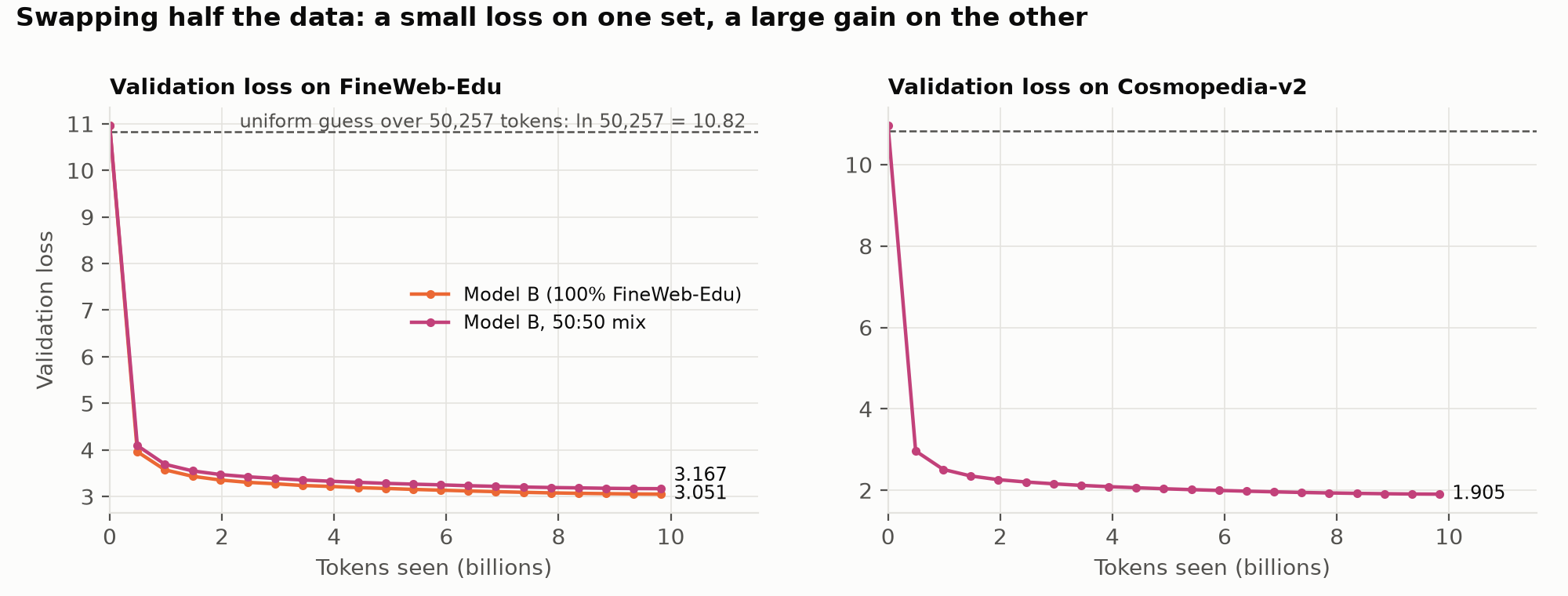
<p>Each dataset is read in order, so the 4.9B FineWeb-Edu tokens in this run
are exactly the first 4.9B that Model B saw. The
run reports loss on held-out FineWeb-Edu and held-out Cosmopedia-v2 from the start, since loss on FineWeb-Edu alone
would make any change of data look bad.</p>

<p><img src="/assets/s1/data_mix/figures/loss_curves.png" alt="Validation loss on both datasets during training" /></p>

<p>Before the run, I expected ARC-Easy to move most, since Cosmopedia is textbook-style science and
explanation; FineWeb-Edu loss to get worse than Model B’s, because the model sees half as much of it; and Cosmopedia
loss to improve a lot. LAMBADA was the open question. Cosmopedia includes synthetic stories, so it might recover some
of the narrative capability FineWeb-Edu filtered out, or it might not, if synthetic stories don’t use names the way novels
do.</p>

<p>The p-values and confidence intervals compare the 50:50 model with Model B, using the same paired tests as in the
Results section.</p>

<table>
  <thead>
    <tr>
      <th> </th>
      <th>Model B, 100% FineWeb-Edu</th>
      <th>Model B, 50:50</th>
      <th>Change</th>
    </tr>
  </thead>
  <tbody>
    <tr>
      <td>Held-out perplexity, FineWeb-Edu</td>
      <td>21.80</td>
      <td>24.56</td>
      <td>+2.76 (+12.7%), 95% CI [+2.64, +2.89]</td>
    </tr>
    <tr>
      <td>Held-out perplexity, Cosmopedia-v2</td>
      <td>20.49</td>
      <td><strong>6.76</strong></td>
      <td>−13.73 (−67%), 95% CI [−13.97, −13.50]</td>
    </tr>
    <tr>
      <td>HellaSwag (acc_norm)</td>
      <td>32.5</td>
      <td>33.2</td>
      <td>+0.7 pt, p = 0.04</td>
    </tr>
    <tr>
      <td>ARC-Easy (acc)</td>
      <td>51.9</td>
      <td>51.6</td>
      <td>−0.3 pt, p = 0.78</td>
    </tr>
    <tr>
      <td>LAMBADA accuracy</td>
      <td>24.5</td>
      <td><strong>26.9</strong></td>
      <td>+2.3 pt, p &lt; 0.001</td>
    </tr>
  </tbody>
</table>

<p>Giving up half the FineWeb-Edu costs 12.7% in perplexity on FineWeb-Edu, while
perplexity on Cosmopedia drops by two-thirds, to 6.8. Synthetic textbook text is very predictable once a
model has seen some of it, and a model this size learns its style almost completely.</p>

<p>The ARC-Easy prediction was wrong: it didn’t move. One plausible explanation is that FineWeb-Edu already
supplies the kind of grade-school science ARC asks about, so more textbook prose adds little. HellaSwag rose by 0.7
points with p = 0.04, just under the 0.05 bar. But this table runs five tests, and the chance that at least one
crosses 0.05 by luck alone is about 23% (1 − 0.95⁵), so I treat it as a hint, not a result.</p>

<p>LAMBADA is the benchmark that clearly moved: accuracy rose 2.3 points,
and splitting by target word shows where:</p>

<table>
  <thead>
    <tr>
      <th>LAMBADA perplexity on the target</th>
      <th>Capitalized (names)</th>
      <th>Lowercase</th>
    </tr>
  </thead>
  <tbody>
    <tr>
      <td>Model B, 100% FineWeb-Edu</td>
      <td>133.7</td>
      <td>98.5</td>
    </tr>
    <tr>
      <td>Model B, 50:50</td>
      <td><strong>84.1</strong></td>
      <td>115.3</td>
    </tr>
    <tr>
      <td>GPT-2</td>
      <td>27.1</td>
      <td>57.0</td>
    </tr>
  </tbody>
</table>

<p>Cosmopedia’s synthetic stories address characters by
name, so the mixed model got some practice at copying a name from earlier in the passage, the skill FineWeb-Edu
had filtered out. It’s still 3x worse than GPT-2 on names, so synthetic fiction gives back only part
of the skill. Meanwhile the lowercase targets, closer to FineWeb-Edu’s kind of text, got a little worse with
half the FineWeb-Edu gone. With architecture and token budget fixed, swapping half the data moved LAMBADA more than any architectural change in
this article, and in the direction the data’s content predicts.</p>

<p>Larger projects tune data mixtures the same way, with many more runs. SmolLM2 was built on small ablations of
data mixtures, then trained in stages, with each stage’s mixing rates adjusted based on the one before (Allal et al. <a href="#ref-17">[17]</a>). NVIDIA’s two-phase pretraining moves to higher-quality data late in training (Feng et al., 2024) <a href="#ref-18">[18]</a>. A single
50:50 data mixture run is the smallest version of that loop.  Other possible mixture strategies are blends that
changes as training iterations proceed.</p>

<h2 id="what-should-carry-over-and-what-might-not">What should carry over, and what might not</h2>

<p>Some of these findings follow from arithmetic and hold at any size; others are specific to 124M models and 1024-token contexts:</p>

<table>
  <thead>
    <tr>
      <th>Finding at 124M</th>
      <th>With bigger models</th>
      <th>With longer contexts</th>
      <th>Grounded in</th>
    </tr>
  </thead>
  <tbody>
    <tr>
      <td>The architectures tie on loss; RoPE helps early</td>
      <td>Unknown from these runs; the papers report GQA and local windows as close to quality-neutral by design</td>
      <td>Local windows risk long-range quality; global layers carry it</td>
      <td>Papers; the rest is open</td>
    </tr>
    <tr>
      <td>Output layer is ~30% of FLOPs, attention ~7%</td>
      <td>Output layer falls to a few percent</td>
      <td>Attention surpasses the MLP at \(T ≈ 8d\)</td>
      <td>Arithmetic</td>
    </tr>
    <tr>
      <td>Model B trains 4% slower despite fewer FLOPs</td>
      <td>The gap should shrink: its extra work grows with \(d\), matmuls with \(d^2\)</td>
      <td>Local windows start saving real FLOPs, given a kernel that skips masked blocks</td>
      <td>Arithmetic + kernel behaviour</td>
    </tr>
    <tr>
      <td>Data can be more important than architecture for certain capabilities</td>
      <td>No reason to expect scale alone to fix a data gap</td>
      <td>—</td>
      <td>Our runs + Olsson et al. 2022 <a href="#ref-13">[13]</a></td>
    </tr>
    <tr>
      <td>Most benchmarks sit near chance</td>
      <td>They become informative, and paired tests matter more, since differences between strong models are small</td>
      <td>—</td>
      <td>Published results</td>
    </tr>
    <tr>
      <td>Plain data parallelism: every GPU holds the whole model and optimizer</td>
      <td>Tops out at ~4.5B parameters per 80 GB GPU (about 17 bytes per parameter); larger needs state sharding</td>
      <td>—</td>
      <td>Arithmetic (ZeRO <a href="#ref-10">[10]</a>)</td>
    </tr>
    <tr>
      <td>Run resume, storage and data replay need care</td>
      <td>More critical: ~84 GB checkpoints at 7B; spikes need precise batch skipping</td>
      <td>—</td>
      <td>Arithmetic + PaLM <a href="#ref-11">[11]</a></td>
    </tr>
  </tbody>
</table>

<h2 id="acknowledgement">Acknowledgement</h2>
<p>Thanks for reading through my work and findings! If you spot a mistake, or have comments or critiques, I’d be glad to
hear them: please reach out on <a href="https://www.linkedin.com/in/shinibali-bhattacharyya/">LinkedIn</a> or <a href="https://x.com/ShinibaliB">X</a>.</p>

<p>This article leans on people who explained things well and acted as my knowledge base:</p>

<ul>
  <li><strong>Andrej Karpathy:</strong> <a href="https://github.com/karpathy/nanoGPT">nanoGPT</a>,
<a href="https://github.com/karpathy/build-nanogpt">build-nanogpt and <em>Let’s reproduce GPT-2 (124M)</em></a>, and
<a href="https://github.com/karpathy/llm.c">llm.c</a>.
The llm.c discussions are where the GPT-2 HellaSwag reference numbers come from.</li>
  <li><strong>Aleksa Gordić:</strong> <a href="https://www.aleksagordic.com/blog/transformer"><em>Inside the Transformer: The Life of a Token</em></a>.
It’s the reason Model B is Gemma 3-style, and it’s the article to go to for an illustrated understanding
of RoPE, YaRN, GeGLU, RMSNorm and hybrid local/global attention.</li>
  <li><strong>Percy Liang and Tatsunori Hashimoto:</strong> Stanford’s <a href="https://cs336.stanford.edu/"><em>CS336: Language Modeling from Scratch</em></a>.
Its lectures are a big part of how I learned the material behind this series.</li>
  <li><strong>Horace He:</strong> <a href="https://horace.io/brrr_intro.html"><em>Making Deep Learning Go Brrrr From First Principles</em></a>. It’s the
lens for every speed number here: whether an operation is limited by compute, memory bandwidth or overhead.</li>
  <li><strong>Hugging Face:</strong> <a href="https://huggingfacetb-smol-training-playbook.hf.space/"><em>The Smol Training Playbook</em></a>, on running
ablations and training at the scale of hundreds of GPUs, and the
<a href="https://arxiv.org/abs/2406.17557">FineWeb</a> and SmolLM teams for FineWeb-Edu and Cosmopedia, the data both models
learned from.</li>
</ul>

<p>Platforms and tools I used:</p>

<ul>
  <li>I rented the H100 GPUs for every training run by the hour on <a href="https://www.runpod.io/">RunPod</a>.</li>
  <li><a href="https://wandb.ai/">Weights &amp; Biases</a> logged every run. Most of the figures here are rebuilt from those logs.</li>
  <li><a href="https://huggingface.co/">Hugging Face Hub</a> stored the model checkpoints and the tokenized shards.</li>
  <li>EleutherAI’s <a href="https://github.com/EleutherAI/lm-evaluation-harness">lm-evaluation-harness</a> ran every benchmark.</li>
  <li><a href="https://claude.com/claude-code">Claude Code</a>, Anthropic’s coding assistant, worked alongside me throughout: it guided the GPU pod setup and checked each run, helped me debug when I was stuck, wrote the analysis and plotting scripts, and helped draft and fact-check this article.</li>
</ul>

<h2 id="appendix">Appendix</h2>

<h3 id="counting-the-flops">Counting the FLOPs</h3>

<p>The forward FLOPs per token, from applying the \(2mn\) rule to every matrix multiplication in a layer: the linear projections and the attention computation itself. Multiplying an \(m\)-dimensional vector by an \(m × n\) matrix costs \(2mn\) FLOPs, one multiply and one add per weight. Everything else (biases, normalization, activations, softmax, RoPE’s rotations, residual additions, the embedding lookup and the loss) is left out, since together it comes to under 1% of the FLOPs.</p>

<table>
  <thead>
    <tr>
      <th>Symbol</th>
      <th>Meaning</th>
      <th>Model A</th>
      <th>Model B</th>
    </tr>
  </thead>
  <tbody>
    <tr>
      <td>\(d\)</td>
      <td>model dimension (\(d_{model}\)): the size of each token’s vector</td>
      <td>768</td>
      <td>768</td>
    </tr>
    <tr>
      <td>\(L\)</td>
      <td>layers (global + local)</td>
      <td>12 (12 + 0)</td>
      <td>12 (3 + 9)</td>
    </tr>
    <tr>
      <td>\(L_{\text{global}}, L_{\text{local}}\)</td>
      <td>global layers, local layers</td>
      <td>12, 0</td>
      <td>3, 9</td>
    </tr>
    <tr>
      <td>\(n_h, n_{kv}\)</td>
      <td>query heads, key/value heads</td>
      <td>12, 12</td>
      <td>12, 3</td>
    </tr>
    <tr>
      <td>\(h = d / n_h\)</td>
      <td>head size</td>
      <td>64</td>
      <td>64</td>
    </tr>
    <tr>
      <td>\(T\)</td>
      <td>context length</td>
      <td>1024</td>
      <td>1024</td>
    </tr>
    <tr>
      <td>\(W\)</td>
      <td>local window</td>
      <td>—</td>
      <td>512</td>
    </tr>
    <tr>
      <td>\(V\)</td>
      <td>vocabulary (padded)</td>
      <td>50,304</td>
      <td>50,304</td>
    </tr>
  </tbody>
</table>

<p>Per layer, per token:</p>

<table>
  <thead>
    <tr>
      <th>Piece</th>
      <th>FLOPs</th>
      <th>Model A</th>
      <th>Model B</th>
    </tr>
  </thead>
  <tbody>
    <tr>
      <td>Q, K, V projections</td>
      <td>\(2d^2 + 2d·(2n_{kv}·h)\)</td>
      <td>\(6d^2\)</td>
      <td>\(3d^2\) (GQA, \(n_h : n_{kv} = 4:1\))</td>
    </tr>
    <tr>
      <td>Attention output projection</td>
      <td>\(2d^2\)</td>
      <td>\(2d^2\)</td>
      <td>\(2d^2\)</td>
    </tr>
    <tr>
      <td>MLP</td>
      <td>GELU: \(2(d·4d + 4d·d)\); GeGLU: \(2(d·2f + f·d)\) with \(f = 8d/3\)</td>
      <td>\(16d^2\)</td>
      <td>\(16d^2\)</td>
    </tr>
    <tr>
      <td>Attention scores \(q·k\) + weighted sum of \(v\)</td>
      <td>\(4d·k̄\)</td>
      <td>\(4d·(T + 1)/2\)</td>
      <td>same in global layers; \(4d·k̄_W\) in local ones</td>
    </tr>
  </tbody>
</table>

<p>Here \(k̄\) is the number of keys a query sees, averaged over positions. With causal masking, position \(p\) sees \(p + 1\)
keys, so a global layer averages \((T + 1)/2\). A local layer ramps up to \(W\) keys and then stays there, so \(k̄_W = [W(W + 1)/2 + (T − W)·W] / T\).
For each key it sees, a query does two length-\(d\) operations across its heads: the dot product \(q·k\) (\(d\)
multiplies and \(d\) adds, so \(2d\) FLOPs) and adding that key’s weighted value to the output (another \(2d\)), so
attention costs \(4d\) FLOPs per key. GQA doesn’t change this, since every query head still does its own dot products.
Summed over a whole sequence, this per-token cost becomes attention’s familiar quadratic; <a href="https://shinibali.github.io/gpt2-to-gemma-part-2/#attention-and-flashattention">Part 2’s appendix</a> works that out, along with what FlashAttention and local windows change at long contexts.</p>

<p>Once per token, the output layer adds \(2dV\) FLOPs.</p>

<p>Adding it up, the weight matrices cost \(6d^2 + 2d^2 + 16d^2 = 24d^2\) per layer in Model A and \(3d^2 + 2d^2 + 16d^2 = 21d^2\) in Model B:</p>

\[F_A = L\,\big(24d^2 + 2d(T+1)\big) + 2dV\]

\[F_B = 21\,L\,d^2 + 2d(T+1)\,L_{\text{global}} + 4d\,\bar{k}_W\,L_{\text{local}} + 2dV\]

<p>The \(21d^2\) assumes Model B’s four query heads per key/value head, so \(n_{kv}·h = d/4\). With other ratios, the projection
term is \(2d(d + 2·n_{kv}·h) + 2d^2\).</p>

<p>Plugging in the numbers:</p>

<ul>
  <li>Model A: \(12 × (14.16M + 1.57M) + 77.27M = 266.0M\) FLOPs per token.</li>
  <li>Model B: \(12 × 12.39M + 3 × 1.57M + 9 × 1.18M + 77.27M = 241.2M\) FLOPs per token (\(k̄_W = 384.25\)).</li>
</ul>

<h3 id="reproducing-this-article">Reproducing this article</h3>

<p>The trained models are public on Hugging Face, each with a model card:
<a href="https://huggingface.co/CuriosLM/gpt2-124m-fineweb-edu">Model A</a>, in the standard 🤗 transformers GPT-2 format;
<a href="https://huggingface.co/CuriosLM/gemma-style-113m-fineweb-edu">Model B</a>; and
<a href="https://huggingface.co/CuriosLM/gemma-style-113m-fineweb-edu-cosmopedia">Model B on the 50:50 mix</a>.</p>

<p>The code for training, evaluation and every figure is in the <a href="https://github.com/Shinibali/CuriosLM">CuriosLM repository</a>,
and its README explains how to run each part.</p>

<h3 id="compute-and-cost">Compute and cost</h3>

<table>
  <thead>
    <tr>
      <th>Session</th>
      <th>Runs</th>
      <th>Hardware</th>
      <th>Training time</th>
      <th>Cost</th>
    </tr>
  </thead>
  <tbody>
    <tr>
      <td>First pods</td>
      <td>Setup and smoke tests</td>
      <td>—</td>
      <td>—</td>
      <td>$4.01</td>
    </tr>
    <tr>
      <td>Calibration and ladder</td>
      <td>Micro-batch calibration; 5 rungs × 1.5B tokens</td>
      <td>2× H100 SXM</td>
      <td>~2.5 h (ladder)</td>
      <td>$22.36</td>
    </tr>
    <tr>
      <td>Seed rerun and headline</td>
      <td>Rung a4 with a second seed; Models A and B, 9.8B tokens each</td>
      <td>2× then 4× H100 SXM</td>
      <td>0.5 h; 1.6 h + 1.7 h</td>
      <td>$51.94</td>
    </tr>
    <tr>
      <td>Data mix</td>
      <td>Model B on the 50:50 mix, 9.8B tokens; smoke test; H100 inference benchmark (Part 2)</td>
      <td>4× H100 SXM</td>
      <td>1.7 h</td>
      <td>$29.49</td>
    </tr>
    <tr>
      <td>YaRN</td>
      <td>Smoke test; 200-step fine-tune (Part 2)</td>
      <td>1× H100 SXM</td>
      <td>~0.4 h</td>
      <td>$2.07</td>
    </tr>
    <tr>
      <td><strong>Total</strong></td>
      <td> </td>
      <td> </td>
      <td> </td>
      <td><strong>$109.87</strong></td>
    </tr>
  </tbody>
</table>

<h3 id="what-broke-during-training-and-how-i-fixed-it">What broke during training and how I fixed it</h3>

<p>None of the results above came out of a clean first attempt. These are the failures that cost real time or money, in no particular order:</p>

<ul>
  <li>
    <p><strong>Resumed runs weren’t exact:</strong> A run that stops and restarts should be indistinguishable from one that never stopped. After the first resume, the
loss dropped from 10.2 to 9.7 in a few steps, suspiciously fast: the model was seeing data it had already trained
on. Three separate bugs were behind it:</p>

    <ul>
      <li>The data loader’s position wasn’t saved in the checkpoint, so a resumed run started the data over.</li>
      <li>The batch the loader had already fetched ahead of time was skipped on restart.</li>
      <li>Evaluation was drawing its batches from the training stream, which shifted where training read next.</li>
    </ul>

    <p>The fixes: save the loader’s state with the checkpoint, restore the prefetched batch, and give evaluation
its own fixed batches. A test now stops a run, resumes it, and checks it matches an uninterrupted run bit for bit.</p>
  </li>
  <li>
    <p><strong>Local attention made training slower:</strong> The first version of rung a4 trained 9% <em>slower</em> than the rung before it, because the
window, written as a dense mask, knocked attention off its FlashAttention path. FlexAttention’s block masks won back
about 5%, and brought problems of their own. FlexAttention has no backward pass on Apple GPUs or CPUs, so it only runs
on CUDA under <code class="language-plaintext highlighter-rouge">torch.compile</code>, with the dense mask as the fallback; both paths read the window rule from one shared
function, so they can’t disagree. Along the way, the mask got built as a tensor instead of a function, FlexAttention
got applied to the <em>global</em> layers too, and a mask buffer was never registered. Unit tests caught all three.</p>
  </li>
  <li>
    <p><strong>The data mix alternated by optimizer step:</strong> The 50:50 run blends two datasets micro-batch by micro-batch. The first version of the blending loader decided the
mix the same way on every GPU. On one GPU that’s correct. On 8 GPUs, all eight would read FineWeb-Edu on the same
micro-step, then all eight would read Cosmopedia on the next: every <em>optimizer step</em> would have been 100% one dataset
or the other, alternating. The fix numbers the micro-batches globally across GPUs and runs Megatron-LM’s blending rule
over that global sequence. Every step is now exactly 50:50 on 1, 2, 4 or 8 GPUs, and the tests check each
count.</p>
  </li>
  <li>
    <p><strong>MMLU took three hours on the Mac:</strong> Before setting MMLU aside, I ran it once to check whether a model this size could beat chance. That
run crawled on the M1 Pro, while HellaSwag had been fast. The process had grown to 17 GB and was swapping to
disk. MMLU’s prompts are long, and scoring needs the full-vocabulary logits: one batch of 16 prompts × 1024 positions ×
50,304 vocabulary entries × 4 bytes is 3.3 GB. The log-softmax made a second copy and the model’s own loss
computation a third. HellaSwag’s short prompts never got close. A batch size of 4 fixed it; the better fix is to keep only the rows that are actually scored. Smoke tests should use the <em>longest</em> inputs instead of some random or first few samples.</p>
  </li>
  <li>
    <p><strong>NCCL failure at pod startup:</strong> The first 2-GPU launch on RunPod died before training even started, with
<code class="language-plaintext highlighter-rouge">Failed to bind NVLink SHARP (NVLS) Multicast memory … CUDA error 401</code>. NVLS is an NCCL feature that some hosts don’t
support when you rent a slice of an 8-GPU machine. Some hosts were fine; the 50:50 run’s 4-GPU pod hit it again. Setting
<code class="language-plaintext highlighter-rouge">NCCL_NVLS_ENABLE=0</code> turns the feature off, which costs nothing at 2–4 GPUs and doesn’t change the math.</p>
  </li>
</ul>

<p>These problems grow with model size. Our checkpoints are 12 bytes per parameter (float32 weights plus Adam’s two
moment estimates). For comparison, a 7B checkpoint would be about 84 GB, close to our CuriosLM Hugging Face org’s entire 100 GB cap. The same habits apply at any size: smoke-test every machine, verify every checkpoint, make the data order replayable.</p>

<h2 id="references">References</h2>

<ol>
  <li><span id="ref-1"></span>Radford et al. (2019). <a href="https://cdn.openai.com/better-language-models/language_models_are_unsupervised_multitask_learners.pdf">Language Models are Unsupervised Multitask Learners</a>.</li>
  <li><span id="ref-2"></span>Brown et al. (2020). <a href="https://arxiv.org/abs/2005.14165">Language Models are Few-Shot Learners</a>.</li>
  <li><span id="ref-3"></span>Su et al. (2021). <a href="https://arxiv.org/abs/2104.09864">RoFormer: Enhanced Transformer with Rotary Position Embedding</a>.</li>
  <li><span id="ref-4"></span>Ainslie et al. (2023). <a href="https://arxiv.org/abs/2305.13245">GQA: Training Generalized Multi-Query Transformer Models from Multi-Head Checkpoints</a>.</li>
  <li><span id="ref-5"></span>Shazeer (2020). <a href="https://arxiv.org/abs/2002.05202">GLU Variants Improve Transformer</a>.</li>
  <li><span id="ref-6"></span>Zhang &amp; Sennrich (2019). <a href="https://arxiv.org/abs/1910.07467">Root Mean Square Layer Normalization</a>.</li>
  <li><span id="ref-7"></span>Gemma Team (2024). <a href="https://arxiv.org/abs/2408.00118">Gemma 2: Improving Open Language Models at a Practical Size</a>.</li>
  <li><span id="ref-8"></span>Gemma Team (2025). <a href="https://arxiv.org/abs/2503.19786">Gemma 3 Technical Report</a>.</li>
  <li><span id="ref-9"></span>Hoffmann et al. (2022). <a href="https://arxiv.org/abs/2203.15556">Training Compute-Optimal Large Language Models</a>.</li>
  <li><span id="ref-10"></span>Rajbhandari et al. (2019). <a href="https://arxiv.org/abs/1910.02054">ZeRO: Memory Optimizations Toward Training Trillion Parameter Models</a>.</li>
  <li><span id="ref-11"></span>Chowdhery et al. (2022). <a href="https://arxiv.org/abs/2204.02311">PaLM: Scaling Language Modeling with Pathways</a>.</li>
  <li><span id="ref-12"></span>Shoeybi et al. (2019). <a href="https://arxiv.org/abs/1909.08053">Megatron-LM: Training Multi-Billion Parameter Language Models Using Model Parallelism</a>.</li>
  <li><span id="ref-13"></span>Olsson et al. (2022). <a href="https://arxiv.org/abs/2209.11895">In-context Learning and Induction Heads</a>.</li>
  <li><span id="ref-14"></span>Dao et al. (2022). <a href="https://arxiv.org/abs/2205.14135">FlashAttention: Fast and Memory-Efficient Exact Attention with IO-Awareness</a>.</li>
  <li><span id="ref-15"></span>Dong et al. (2024). <a href="https://arxiv.org/abs/2412.05496">Flex Attention: A Programming Model for Generating Optimized Attention Kernels</a>.</li>
  <li><span id="ref-16"></span>Penedo et al. (2024). <a href="https://arxiv.org/abs/2406.17557">The FineWeb Datasets: Decanting the Web for the Finest Text Data at Scale</a>.</li>
  <li><span id="ref-17"></span>Allal et al. (2025). <a href="https://arxiv.org/abs/2502.02737">SmolLM2: When Smol Goes Big — Data-Centric Training of a Small Language Model</a>.</li>
  <li><span id="ref-18"></span>Feng et al. (2024). <a href="https://arxiv.org/abs/2412.15285">Maximize Your Data’s Potential: Enhancing LLM Accuracy with Two-Phase Pretraining</a>.</li>
  <li><span id="ref-19"></span>Zellers et al. (2019). <a href="https://arxiv.org/abs/1905.07830">HellaSwag: Can a Machine Really Finish Your Sentence?</a>.</li>
  <li><span id="ref-20"></span>Clark et al. (2018). <a href="https://arxiv.org/abs/1803.05457">Think you have Solved Question Answering? Try ARC, the AI2 Reasoning Challenge</a>.</li>
  <li><span id="ref-21"></span>Paperno et al. (2016). <a href="https://arxiv.org/abs/1606.06031">The LAMBADA dataset: Word prediction requiring a broad discourse context</a>.</li>
  <li><span id="ref-22"></span>Miller (2024). <a href="https://arxiv.org/abs/2411.00640">Adding Error Bars to Evals: A Statistical Approach to Language Model Evaluations</a>.</li>
  <li><span id="ref-23"></span>McNemar (1947). Note on the sampling error of the difference between correlated proportions or percentages. <em>Psychometrika</em> 12(2), 153–157. <a href="https://doi.org/10.1007/BF02295996">doi:10.1007/BF02295996</a>.</li>
  <li><span id="ref-24"></span>Efron (1979). Bootstrap Methods: Another Look at the Jackknife. <em>Annals of Statistics</em> 7(1), 1–26. <a href="https://doi.org/10.1214/aos/1176344552">doi:10.1214/aos/1176344552</a>.</li>
  <li><span id="ref-25"></span>Korthikanti et al. (2022). <a href="https://arxiv.org/abs/2205.05198">Reducing Activation Recomputation in Large Transformer Models</a>.</li>
  <li><span id="ref-26"></span>NVIDIA. <a href="https://docs.nvidia.com/deeplearning/performance/dl-performance-matrix-multiplication/index.html">Matrix Multiplication Background User’s Guide</a>, sections “Tensor Core Requirements” and “Tile Quantization”.</li>
  <li><span id="ref-27"></span>Ding et al. (2021). <a href="https://arxiv.org/abs/2105.13290">CogView: Mastering Text-to-Image Generation via Transformers</a>.</li>
</ol>

<h2 id="citation">Citation</h2>

<div class="language-bibtex highlighter-rouge"><div class="highlight"><pre class="highlight"><code><span class="nc">@misc</span><span class="p">{</span><span class="nl">bhattacharyya2026gpt_to_gemma_1</span><span class="p">,</span>
  <span class="na">author</span>       <span class="p">=</span> <span class="s">{Bhattacharyya, Shinibali}</span><span class="p">,</span>
  <span class="na">title</span>        <span class="p">=</span> <span class="s">{GPT-2 (124M) to Gemma 3-Style (113M) language models, Part 1: Pretraining lessons from swapping one architecture component at a time}</span><span class="p">,</span>
  <span class="na">year</span>         <span class="p">=</span> <span class="s">{2026}</span><span class="p">,</span>
  <span class="na">url</span>          <span class="p">=</span> <span class="s">{https://shinibali.github.io/gpt2-to-gemma-part-1/}</span><span class="p">,</span>
<span class="p">}</span>
</code></pre></div></div>]]></content><author><name>Shinibali Bhattacharyya</name></author><summary type="html"><![CDATA[In this article, I will share what I learned from pretraining language models from scratch, and how to build intuition about their inner workings as model architecture and parameter count change. Thanks to epic learning resources available on the internet, I started with Andrej Karpathy’s nanoGPT project Let’s reproduce GPT-2 (124M). I also got inspired by Aleksa Gordić’s awesome illustrative article Inside the Transformer: The Life of a Token, where he walks through Essential AI’s Rnj-1.5 7B model, which closely follow the Gemma 3 architecture and uses YaRN to stretch its context window. It explains grouped-query attention (GQA), rotary position embeddings (RoPE), YaRN, gated MLPs (GeGLU), RMSNorm and hybrid local/global attention so clearly that I wanted to find out: what do these architecture choices actually buy when you train models at the scale I had started at, and how does data affect what the models can do?]]></summary></entry><entry><title type="html">GPT-2 (124M) to Gemma 3-Style (113M) language models, Part 2: KV caches, RoPE clocks, 4× context extension and attention visualization</title><link href="https://shinibali.github.io/gpt2-to-gemma-part-2/" rel="alternate" type="text/html" title="GPT-2 (124M) to Gemma 3-Style (113M) language models, Part 2: KV caches, RoPE clocks, 4× context extension and attention visualization" /><published>2026-10-14T00:00:00+00:00</published><updated>2026-10-14T00:00:00+00:00</updated><id>https://shinibali.github.io/gpt2-to-gemma-part-2</id><content type="html" xml:base="https://shinibali.github.io/gpt2-to-gemma-part-2/"><![CDATA[<p>This is the second part of my GPT-2 to Gemma 3-style language model series. In <a href="/gpt2-to-gemma-part-1/">Part 1</a>, I trained a GPT-2 124M (Model A) and a
Gemma 3-style 113M model (Model B) on the same 9.8 billion tokens and found them tied on quality, with the
Gemma recipe slightly slower to train but with a 6.4× smaller KV cache. In this part, I look at the model internals at inference time: how
fast they generate text and how they represent position. I then extend Model B’s context length from 1024 to 4096
tokens with YaRN, and finally look at what each model attends to.</p>

<p>Here is the TLDR of what I found:</p>

<ul>
  <li>On my M1 Pro MacBook, whose memory bandwidth is about 1/17 of an H100’s, Model B generates text up to 1.55× faster
than Model A due to its 6.4× smaller KV cache. But on an H100, Model B is 1/3 slower than A. At this size, the H100 spends most of each step on the fixed cost of launching
GPU operations, and Model B has more of them. So the smaller cache size pays off at serving scale, with big
batches, long contexts and bigger models.</li>
  <li>RoPE gives Model B 32 fixed “clocks” to read position from: pairs of dimensions that rotate at different speeds as
the position grows. Model A’s learned position table organizes itself into slow waves instead. The two schemes work
differently, but in both models, how similar two positions look depends mainly on how far apart they are.</li>
  <li>YaRN helped stretch Model B from 1024 to 4096 tokens (4×) with no retraining, taking perplexity at 4096 from 37.7 down to
23.2. Continuing the training run for 200 steps (1% of pretraining) brings perplexity to 21.0, close to the original model’s
20.6 at 1024 tokens.</li>
  <li>Model B’s strongest induction head, the circuit that copies text from earlier in the context, sits in a local layer.
So when the text to copy is, for example, 768 tokens back, Model A still copies it and Model B can’t. On ordinary text the two models
rarely disagree.</li>
</ul>

<h2 id="the-two-models">The two models</h2>

<p>As a reminder, the two models from Part 1 (124M and 113M parameters, 1024 context length) were trained identically on FineWeb-Edu:</p>

<ul>
  <li><strong>Model A</strong> is GPT-2 as nanoGPT ships it: learned position embeddings and full multi-head attention in every layer.</li>
  <li><strong>Model B</strong> is Gemma 3-style <a href="#ref-9">[9]</a>: RoPE <a href="#ref-1">[1]</a>, grouped-query attention (12 query heads sharing 3 key/value heads), a GeGLU MLP,
sandwich RMSNorm, and local 512-token attention in three layers out of four.</li>
</ul>

<p>The two models tied on loss and on every benchmark. On paper, Model B needs fewer FLOPs; in practice, it trained 4% slower. Most of the Gemma recipe targets efficiency and longer contexts. Its two attention changes, GQA and local windows,
shrink the memory a model needs during inference, and RoPE makes position relative and easier to extend to
longer contexts.</p>

<h2 id="generating-text-with-a-kv-cache">Generating text with a KV cache</h2>

<p>To measure how the smaller cache helps during text generation, I benchmarked both models with a KV cache on two kinds of hardware. The answer turned out to depend more
on the hardware than on the model.</p>

<h3 id="what-a-kv-cache-stores">What a KV cache stores</h3>

<p>A language model generates one token at a time, and each new token attends to every token before it. Without a cache,
every step reprocesses the whole sequence from scratch, which is wasteful because the keys and values of earlier
tokens never change. A KV cache stores them once and reuses them, so each step only has to process  one new token.
Queries aren’t cached because in a causal model, each token’s query is used only once, to compute that token’s own
output, which later tokens can never change. Only keys and values are read again by every token that comes after.</p>

<p>Each layer stores one key and one value (the 2 below) per key/value head and per cached position, so the cache for
one sequence takes</p>

\[\text{KV cache bytes} = 2 \cdot n_{kv} \cdot h \cdot b \cdot \sum_{\ell=1}^{L} T_\ell\]

<p>where:</p>

<ul>
  <li>Number of key/value heads, \(n_{kv}\): 12 in Model A, 3 in Model B.</li>
  <li>Head size, \(h\): each key and each value is a vector of 64 numbers.</li>
  <li>Bytes per number, \(b\): 4 in float32, 2 in bf16.</li>
  <li>Number of layers, \(L\): 12 in both models.</li>
  <li>Positions kept by layer \(\ell\), \(T_\ell\): how many past tokens that layer holds keys and values for. A global
layer keeps every 1024 token; a local layer keeps at most 511.</li>
</ul>

<p>Model A keeps all 12 heads for all 1024 positions in all
12 layers: 75.5 MB. Model B keeps only its 3 key/value heads, which its 12 query heads share, a 4x saving. Its local
layers never look further back than their window, so 9 of its 12 layers stop at 511 positions. Together that’s
11.8 MB, 6.4x smaller.</p>

<h3 id="what-limits-generation-speed">What limits generation speed</h3>

<p>Horace He’s <a href="https://horace.io/brrr_intro.html"><em>Making Deep Learning Go Brrrr</em></a> <a href="#ref-12">[12]</a> sorts GPU time by what the chip is waiting on:</p>

<ul>
  <li><strong>Compute:</strong> matrix multiplications and element-wise operations.</li>
  <li><strong>Memory bandwidth:</strong> it’s waiting for data to arrive from memory.</li>
  <li><strong>Overhead:</strong> it’s waiting for the next instruction. That covers launching kernels, Python, and moving small
tensors around.</li>
</ul>

<p>Which of these dominates decides whether a smaller KV cache makes a model faster. Generating text with a KV cache
happens in two phases, prefill and decode, and each runs into a different limit.</p>

<p><strong>Prefill</strong> reads the prompt: every prompt token goes through the model in one forward pass, and their keys and values
are <em>written</em> to the cache. With enough tokens (many batches and long context length), that’s large matrix multiplications, so prefill leans towards
<em>compute</em>. Its speed depends on number of FLOPs more than on cache size. Model B does 9% less FLOPs per token than Model A (<a href="/gpt2-to-gemma-part-1/#counting-flops">Part 1, “Counting FLOPs”</a>).</p>

<p><strong>Decode</strong> generates the answer one token per step. So each step does very little math, but it has to read every
weight and every sequence’s whole cache. For a large model that makes decode <em>memory-bound</em>, which is where a
smaller cache pays off. For a small model there is overhead cost: each step  pays a fixed cost to launch a few hundred
small kernels, one per operation per layer. If that fixed cost is bigger than the time spent moving data, decode is
<em>overhead-bound</em>, and the cache size barely matters.</p>

<p>If you’ve used an LLM API with “cache write” and “cache read”, that is when prefill writes the KV cache and
decode reads it.</p>

<h3 id="mac-vs-h100">Mac vs H100</h3>

<p>I ran the same benchmark on my M1 Pro MacBook (16-core GPU, 16 GB of unified memory, 200 GB/s memory bandwidth) and on
one H100 SXM (80 GB of HBM3 memory, 3.35 TB/s memory bandwidth), both in float32 (the model checkpoints’ precision), taking the median of repeated runs after warm-up. Each generation run starts from a
prompt of random token IDs and produces 256 new tokens, always
picking the most likely next one. I used random tokens because the content of a prompt doesn’t affect how fast the model generates.</p>

<table>
  <thead>
    <tr>
      <th> </th>
      <th>Model A</th>
      <th>Model B</th>
      <th>B vs A</th>
    </tr>
  </thead>
  <tbody>
    <tr>
      <td>KV cache per sequence, 1024 tokens (any machine)</td>
      <td>75.5 MB</td>
      <td>11.8 MB</td>
      <td>6.4× smaller</td>
    </tr>
    <tr>
      <td><strong>Mac:</strong> decode with cache, batch 8, 512-token prompt</td>
      <td>297 tok/s</td>
      <td>461 tok/s</td>
      <td><strong>1.55×</strong></td>
    </tr>
    <tr>
      <td><strong>Mac:</strong> prefill, batch 8, 1024 tokens</td>
      <td>13.5k tok/s</td>
      <td>12.2k tok/s</td>
      <td>0.90×</td>
    </tr>
    <tr>
      <td><strong>H100:</strong> decode with cache, batch 8, 512-token prompt</td>
      <td>1,988 tok/s</td>
      <td>1,290 tok/s</td>
      <td><strong>0.65×</strong></td>
    </tr>
    <tr>
      <td><strong>H100:</strong> prefill, batch 8, 1024 tokens</td>
      <td>212k tok/s</td>
      <td>194k tok/s</td>
      <td>0.92×</td>
    </tr>
  </tbody>
</table>

<p>At 1024 tokens, compute-heavy prefill behaves the same on both machines: B is 8–10% slower, in line with Part 1’s training slowdown. On the H100, short batch \(B=1\) prompts are even slower, because they are overhead-bound. The two machines differ substantially in decoding speed. The time per decode step shows why:</p>

<p><img src="/assets/s1/efficiency/figures/decode_regimes.png" alt="Decode step time against megabytes read per step, on each machine" /></p>

<p><strong>Understanding the plots above:</strong> I benchmarked four settings per model: a batch of 1 or 8, each
generating after a 128-token or a 512-token prompt. That’s why each line has four points. The x-axis is how much data
one decode step reads from memory: all the model’s weights, read once and shared by the batch, plus the KV cache of
every sequence in the batch. A bigger batch or a longer sequence means more cache, so the point moves right. The y-axis
shows how long one step takes.</p>

<p><strong>On the Mac (the left plot), step time rises with the data read.</strong> Model A’s step time climbs from about 10 ms to 27 ms as the data
read per step grows from about 520 to 875 MB. Across all eight points of both models, the MB read during decoding
explains the variation in step time. This is what memory-bound looks like: each step mostly waits for the
weights and the cache to arrive. Model B reads less cache per step, so its points sit kind-of-clustered and further left on the x-axis compared to A’s. It’s faster than
Model A in every setting except the smallest one (batch 1, 128-token prompt), where both caches are tiny, and its lead
grows with the batch.</p>

<p><strong>On the H100 (the right plot), step time is flat.</strong> Model A takes 3.8–4.0 ms per step and Model B 6.1–6.3 ms, whatever the batch
and prompt length. The data read barely matters here: at the H100’s 3.35 TB/s, reading 460–880 MB takes only
0.14–0.26 ms. The rest of each step is overhead. A decode step runs a few hundred small GPU operations (kernels), and
launching each one costs a few microseconds, which adds up to milliseconds. Model B runs more of them per block: two
extra normalizations, the gating multiply in its MLP, the rotations and the local-window masks. So on the H100 it’s
slower, and its smaller cache does not help it win in speed.</p>

<p>The next figure shows how much the cache itself speeds up generation (throughput), on the Mac M1 Pro. In the two left panels, each
model has a light bar (generating without the cache, recomputing every earlier token at each step) and a dark bar
(with the cache), and the label above the dark bar is the speed-up. The right panel is prefill throughput (tokens/s) at batch 8, where the
cache plays no part.</p>

<p><img src="/assets/s1/efficiency/figures/inference_speed.png" alt="Generation speed with and without the cache, and prefill speed, on the Mac" /></p>

<p>On the Mac, the cache speeds up generation 2.5–5.3× at batch 1 and 8–23× at batch 8,
because recomputing the whole sequence every step is a lot of extra work.</p>

<p>On the H100 (not in the figure), at batch 1 with a short prompt,
the cache gives no speed-up at all (0.9–1.0×), because recomputing 128 tokens costs similar launch overhead than
processing one. The cache benefit appears only with longer prompts and bigger batches (up to 6.3× for Model A at batch 8).</p>

<p><img src="/assets/s1/efficiency/figures/kv_cache.png" alt="KV-cache memory as the context grows" /></p>

<p>The memory plot above shows the two savings separately. Model B’s line rises 1/4-th as steeply as Model A’s (GQA), and
flattens past 512 tokens, where its local layers stop adding to the cache due to windowed attention. The measured sizes (dots)
match the KV cache formula from
<a href="#what-a-kv-cache-stores">previous section</a> (lines) exactly, on both machines.</p>

<p>When would the H100 result flip? Model A spends about 4 ms of each step on
overhead. In 4 ms, at its peak bandwidth, the H100 can read 3.35 TB/s × 0.004 s ≈ 13 GB. A full 1024-token sequence takes 75.5 MB of Model A’s float32 cache. So for reading the cache to take as long as the
overhead, a step would have to read about 13 GB of cache: 13.4 GB / 75.5 MB ≈ 177 full-length sequences of Model A’s
float32 cache at once. Real serving systems reach the scale where overhead is no longer the bottleneck, using large batches,
long contexts and bigger models, and they also cut the per-step overhead with CUDA graphs and kernel fusion.</p>

<h3 id="the-kv-cache-of-a-larger-model">The KV cache of a larger model</h3>

<p>Arithmetic intensity, the FLOPs done per byte read, tells which part of decoding can ever become compute-bound. A great reference to check out in this regard is 
CS336’s lectures on <a href="https://cs336.stanford.edu/lectures/?trace=lecture_02">resource accounting</a> and
<a href="https://cs336.stanford.edu/lectures/?trace=lecture_10">inference</a>. For the
weights, each parameter read in bf16 (2 bytes) is used for 2 FLOPs per sequence in the batch, so the intensity is
about the batch size. An H100 does about 295 bf16 FLOPs per byte it can read, so decode only becomes compute-bound
for the weights at batches of a few hundred sequences. Attention over the cache is different. Each cached key and
value is read for one sequence only, and is used by every query head that shares it: \(n_h / n_{kv}\) heads, which is 1 in Model A and 4 in Model B.
That gives an intensity of 1 FLOP per byte for Model A and 4 for Model B. Reading the cache is memory-bound at any scale,
and GQA’s task is to multiply that intensity by the number of query heads per key/value head.</p>

<p>The same formula from <a href="#what-a-kv-cache-stores">‘What a KV cache stores’</a> section gives the KV
cache per sequence of, let’s say, a 7B-class model (32 layers, \(d_{model}\) = 4096, 32 heads of size 128) in bf16:</p>

<table>
  <thead>
    <tr>
      <th>Context</th>
      <th>Full multi-head attention</th>
      <th>GQA (8 KV heads)</th>
      <th>GQA + Gemma 3-style local windows</th>
    </tr>
  </thead>
  <tbody>
    <tr>
      <td>8k tokens</td>
      <td>4.3 GB</td>
      <td>1.1 GB</td>
      <td>0.31 GB</td>
    </tr>
    <tr>
      <td>32k tokens</td>
      <td>17.2 GB</td>
      <td>4.3 GB</td>
      <td>0.91 GB</td>
    </tr>
    <tr>
      <td>128k tokens</td>
      <td>68.7 GB</td>
      <td>17.2 GB</td>
      <td>3.3 GB</td>
    </tr>
  </tbody>
</table>

<p>At 32k tokens, one sequence’s full-attention cache would fill 1/5-th of an 80 GB H100. The Gemma 3-style layout fits
nearly twenty sequences in the same space. Overhead stops dominating too: reading a 7B model’s bf16 weights alone
takes about 4 ms per decode step at 3.35 TB/s (7B parameters × 2 bytes = 14 GB, and 14 GB / 3.35 TB/s ≈ 4.2 ms). That’s the regime
the Gemma 3-style architecture targets, where a 6.4x smaller cache means serving 6.4x more sequences in the same GPU memory. At that scale the Mac
result, where the smaller cache made decoding faster, is the one that carries over to the H100.</p>

<h2 id="flops-at-long-contexts">FLOPs at long contexts</h2>

<p><a href="/gpt2-to-gemma-part-1/#counting-flops">Part 1</a> counted each model’s FLOPs per token, term by term. Attention is the only term that grows
with context length, so the same algebra tells us what long contexts do to a model.</p>

<p>Per layer, attention costs \(2d(T + 1)\) FLOPs per token against the MLP’s \(16d^2\), so <strong>attention overtakes the MLP when \(T ≈ 8d\)</strong>, with \(d\) the model dimension. For our \(d\) of 768 that’s about 6000 tokens; for a larger 7B-class
model (\(d\) = 4096), it happens at about 33000 tokens. A local layer’s queries see at most \(W\) keys, so its attention cost levels off at \(4d·W\) per token. That only reaches the MLP’s \(16d^2\) if \(W &gt; 4d\) (about 3,000 tokens at our \(d\)). So with Model B’s
512-token window the local layers attention costs never cross over; only the global layers do.</p>

<p>To see this in practice, I scaled each recipe from Part 1 up to a 7B-class and a 14B-class
model and calculated the forward FLOPs per token at a 1k and a 128k context. The numbers below are absolute FLOPs per token:</p>

<p><img src="/assets/s1/efficiency/figures/flops_by_context.png" alt="Forward GFLOPs per token for Model A's and Model B's recipes, at two sizes and two context lengths" /></p>

<table>
  <thead>
    <tr>
      <th>Forward GFLOPs per token</th>
      <th>1k context</th>
      <th>128k context</th>
      <th>Attention scores’ share at 128k</th>
    </tr>
  </thead>
  <tbody>
    <tr>
      <td>Model A’s recipe, 6.7B</td>
      <td>13.6</td>
      <td>47.7 (3.5×)</td>
      <td>72%</td>
    </tr>
    <tr>
      <td>Model A’s recipe, 15.4B</td>
      <td>31.2</td>
      <td>95.1 (3.0×)</td>
      <td>68%</td>
    </tr>
    <tr>
      <td>Model B’s recipe, 5.8B</td>
      <td>11.9</td>
      <td>20.5 (1.7×)</td>
      <td>43%</td>
    </tr>
    <tr>
      <td>Model B’s recipe, 13.5B</td>
      <td>27.3</td>
      <td>43.4 (1.6×)</td>
      <td>38%</td>
    </tr>
  </tbody>
</table>

<p>With full attention, stretching the context from 1k to 128k tokens multiplies the work per token by 3–3.5×, almost
all of it attention scores. With Model B’s recipe (512-token windows in three layers of four), the same stretch
costs 1.6–1.7×, because only the global layers pay for the long context. The window stays at 512 tokens however long
the context gets, which is how sliding-window models are built: Gemma 3 keeps its 1024-token window at 128k. A window
that grew with the context, say to half of it, would make the local layers quadratic again and remove most of the
saving. So at 128k tokens, a 13.5B model
built with Gemma 3’s recipe does <em>less</em> work per token than a 6.7B model built with GPT-2’s (43 against 48 GFLOPs).
That’s on top of the memory savings from the KV cache section above. Gemma 3’s report <a href="#ref-9">[9]</a> gives memory as its main reason for going to five
local layers in six at 128k.</p>

<p>The same counting matters for how training efficiency is reported. The PaLM formula (Chowdhery et al., 2022) <a href="#ref-17">[17]</a> behind Part 1’s logged MFU
charges every token for attending to the whole context; a causal layer computes about half of that, and a local
layer only its window. At 1024 tokens, for the 7B-class models above, the formula overstates the work by 2–3%. At
128k tokens it overstates it by 72% for Model A’s recipe and by a factor of 3.9 for Model B’s, because it charges
the local layers for the full 128k they never look at. So an MFU number for a long-context or hybrid-attention run is only meaningful if
you know which FLOP count it assumes.</p>

<h3 id="a-note-on-attentions-quadratic-cost">A note on attention’s quadratic cost</h3>

<p>Per token, attention is linear in context length. And summed over a whole sequence it gives the familiar quadratic,
about \(2d·T^2\) FLOPs per layer. FlashAttention <a href="#ref-11">[11]</a> makes that fit in GPU memory at
long contexts, and enforcing local attention changes the order. The
appendix (<a href="#attention-and-flashattention">Attention and FlashAttention</a>) works through the numbers.</p>

<h2 id="how-each-model-represents-position">How each model represents position</h2>

<p>The two models end with the same loss, but they use very different mechanism for the one thing a
transformer can’t know by itself: where each token sits in the sequence. Model A learns a vector for every position
from scratch. Model B is supplied the position through a fixed rotation. Below, I share how each model handles position information.</p>

<h3 id="rope-as-32-clocks">RoPE as 32 clocks</h3>

<p>Each
layer splits the 768 hidden (embedding) dimensions of its queries and keys across 12 heads, so a head gets 768 / 12 = 64 hidden dimensions. RoPE <a href="#ref-1">[1]</a> splits our 64-dimensional attention head into 32 pairs and rotates each pair by an angle
proportional to the token’s position. Each pair turns at its own speed. When a query and a key score attention, only the
<em>difference</em> of their angles survives, so attention depends only on how far apart two tokens are. Here is a mental model that helps me build intuition about RoPE: each attention head reads the distance between two tokens off a set of 32 clocks running at different speeds.</p>

<p>Here is the simple math behind the wavelengths of the fastest and slowest bands. Counting bands from 1, band \(j\) turns by \(\theta_j = 10000^{-2(j-1)/64}\) radians per
position, where 10,000 is RoPE’s base and wavelength, the number of positions for one full turn, is \(2\pi/\theta_j\). The fastest band, \(j = 1\), turns 1 radian per position, so a full turn takes \(2\pi \approx 6.3\) positions. The slowest, \(j = 32\), turns \(10000^{-62/64} \approx 1/7500\) radians
per position, so a full turn takes \(2\pi \times 7500 \approx 47000\) positions.</p>

<p><img src="/assets/s1/positions/figures/rope_bands.png" alt="Wavelength of each RoPE band against the 1024-token training context" /></p>

<p>As shown in the plot above, only 18 of the 32 clocks complete a full turn within the 1024-token training context. The other 14 never do so during
training, the model only ever sees a fraction of their cycle. At 1024 tokens it is harmless but it becomes a
problem when the model reads longer inputs. I will show how YaRN fixes this, later in this article.</p>

<h3 id="how-an-attention-head-uses-the-clocks">How an attention head uses the clocks</h3>

<p>To see what these rotations do to attention, it helps to treat each pair of dimensions as one complex number. I use \(j\) for the band index below, to keep it apart from the imaginary unit \(\mathrm{i}\).</p>

<p>Take one head, with head size \(h = 64\), and band \(j\): dimensions \(j\) and \(j + h/2\), which RoPE rotates by \(m\theta_j\) at position \(m\), where \(\theta_j\) is the band’s fixed speed. The key at position \(n\) is rotated the same way, by \(n\theta_j\).</p>

<p><strong>Step 1: a rotation is a multiplication.</strong> The RoFormer paper <a href="#ref-1">[1]</a> uses the same complex form. Write the query’s pair as one complex number</p>

\[z_j^q(m) = q_j(m) + \mathrm{i}\,q_{j+h/2}(m),\]

<p>and the key’s as \(z_j^k(n)\). Rotating a 2-D vector by an angle \(\alpha\) is the same as
multiplying its complex number by \(e^{\mathrm{i}\alpha}\). So RoPE turns the query’s pair into \(z_j^q(m)\,e^{\mathrm{i} m \theta_j}\), and the key’s into \(z_j^k(n)\,e^{\mathrm{i} n \theta_j}\).</p>

<p><strong>Step 2: a dot product is the real part of a product.</strong> For two 2-D vectors written as complex numbers \(a\) and \(b\),
their dot product is \(\mathrm{Re}[a\,\bar{b}]\), where \(\bar{b}\) is the complex conjugate. So band \(j\)’s share of the attention score is</p>

\[\frac{1}{\sqrt{h}}\,\mathrm{Re}\Big[\, z_j^q(m)\,e^{\mathrm{i} m \theta_j} \cdot \overline{z_j^k(n)\,e^{\mathrm{i} n \theta_j}} \,\Big]
= \frac{1}{\sqrt{h}}\,\mathrm{Re}\Big[\, z_j^q(m)\,\overline{z_j^k(n)} \; e^{\,\mathrm{i} (m-n)\,\theta_j} \Big]\]

<p>where the two \((q,k)\) rotations combine into one. <strong>Only the difference \(\Delta = m - n\) survives.</strong> This is what makes RoPE relative.</p>

<p><strong>Step 3: separate content from position.</strong> The product \(c_j = z_j^q(m)\,\overline{z_j^k(n)}\) depends only on what the
query and key vectors contain before rotation. Writing it as amplitude and an angle, \(c_j = |c_j|\,e^{\mathrm{i}\varphi_j}\) and summing
over the 32 bands gives the whole score:</p>

\[\text{score}(\Delta) = \frac{1}{\sqrt{h}} \sum_{j=1}^{32} |c_j| \cos\!\big(\Delta\,\theta_j + \varphi_j\big)\]

<p>This attention score can be interpreted as a sum of 32 waves, each a function of the distance \(\Delta\) between two tokens. <strong>The waves’ frequencies \(\theta_j\) are fixed by RoPE. How much of each wave a head uses (amplitude \(|c_j|\)), and where each wave
peaks (phase \(\varphi_j\)), are set by content</strong>, through the query and key weights the head has learned. So each head builds its own
preference for distance by mixing fixed waves, a bit like an equaliser setting the volume of fixed
frequency bands.</p>

<p>A head can choose how it treats distance. Fast waves give a sharp preference for nearby
tokens. Middle waves give a smooth fade over tens to hundreds of tokens. Slow waves never complete a turn within the context, so they
change very little between a key 10 tokens away vs one 900 tokens away. They add roughly the same amount to the score
at every distance.</p>

<p>Do Model B’s trained heads actually split like this? To check, I grouped the bands the way the YaRN paper <a href="#ref-3">[3]</a> does,
by counting how many full turns each band makes within the 1024-token training context:</p>

<ul>
  <li><strong>Fast bands</strong> make 32 turns or more (6 of the 32 bands).</li>
  <li><strong>Middle bands</strong> make between 1 and 32 turns (12 bands).</li>
  <li><strong>Slow bands</strong> never complete a single turn (the other 14).</li>
</ul>

<p>The heatmap below answers this from the trained weights:</p>

<p><span id="fig-band-usage"></span>
<img src="/assets/s1/positions/figures/band_usage.png" alt="Which RoPE bands each of Model B's 144 heads uses, measured from the trained weights" /></p>

<p>Each row is one head (12 per layer, 12 layers) and each column one band, fastest on the left. Each
cell is one head’s \(**q·k**\) weight in one band. The head’s <strong>q·k weight</strong> in band \(j\) is the size of the query and
key projection rows that feed band \(j\) which caps how much the head can use it on any input. Darker means more of
that head’s \(q·k\) weight. The derivation is in the
appendix, <a href="#how-the-band-measures-are-computed">How the band measures are computed</a>.</p>

<p>The
pattern leans toward the slow bands on the right. Its <strong>slow-band weight</strong> sums
that share over the 14 slow bands:</p>

<ul>
  <li><strong>Overall:</strong> the median slow-band weight is 53%, against 44% for an even spread.</li>
  <li><strong>Five heads have a slow-band weight above 75%:</strong> one in layer 1, three in layer 6 and one in layer 8. They’re the
dark stripes on the right.</li>
  <li><strong>No head concentrates on the fast bands.</strong> The lowest slow-band weights, mostly in layer 0, sit at or just below the 44%
of an even spread.</li>
</ul>

<p>This matches what Barbero et al. (2025) <a href="#ref-2">[2]</a> found in a much larger Gemma model: a strong preference for the lowest
frequencies slow bands, which they interpret as carrying meaning, and the highest frequencies fast bands used for positional patterns.</p>

<p>The weights only show what a head <em>can</em> use. The <a href="#fig-real-heads">figure</a> below shows what it <em>does</em> use on real text. I ran held-out
FineWeb-Edu through Model B for three heads, averaging the pre-softmax score \(q·k/\sqrt{h}\) over every query–key pair the
same distance apart. Using the complex form from the derivation above, that average score splits exactly into one contribution per
band (formula in the <a href="#how-the-band-measures-are-computed">appendix</a>). The figure’s bottom row is the head’s mean score at each distance, and the top
row sums the bands’ contributions within each speed group: fast, middle and slow.</p>

<p><span id="fig-real-heads"></span>
<img src="/assets/s1/positions/figures/real_heads.png" alt="Three real Model B heads: average attention score vs distance, and the contribution of fast, middle and slow bands" /></p>

<p>Each column in the above plot is one real head, chosen from the heatmap:</p>

<ul>
  <li>the highest slow-band weight (layer 6, head 11, 84%);</li>
  <li>the median (layer 9, head 1, 53%);</li>
  <li>the lowest (layer 0, head 6, 42%).</li>
</ul>

<p>Panel titles mark global or local layers; local heads’ curves stop at \(W = 512\). Each head matches one of the behaviours described earlier:</p>

<ul>
  <li><strong>Layer 0, head 6 is sharply local.</strong> Its score halves from distance 0 to distance 1 and keeps falling. That first
drop is spread across all three speed groups.</li>
  <li><strong>Layer 9, head 1 fades smoothly</strong> over about 100 tokens, through its middle and slow bands together.</li>
  <li><strong>Layer 6, head 11 barely cares about distance</strong> beyond its immediate neighbours: its score is nearly flat from 3
tokens out to the edge of its 512-token window, and its fast bands contribute nothing at all.</li>
</ul>

<p>One point to note in these plots, they mix two things, RoPE’s rotations and the fact that nearby tokens tend to be
similar in content. The steep drop over the first few tokens in the slow bands, in layer 6’s head and layer 0’s, can’t
come from rotation, since those bands barely turn in a few tokens. It comes from content, that is a query matching keys from its own
neighbourhood. The flat stretch beyond that is where the slow bands’ indifference to position shows.</p>

<h3 id="model-as-learned-position-table">Model A’s learned position table</h3>

<p>Model A’s position table is just 1024 learnt vectors of \(d=768\) dimension each. By its design, there is no encoding about distance, smoothness
or waves information. But training gives it structure. Model B has no such table, since RoPE rotates queries and keys instead
of adding a vector to each token. But one thing can be compared directly between the two models: how similar two positions look as a
function of their distance.</p>

<p>The plot below captures the
cosine similarity between the position vectors \(p_m\) and \(p_n\) at positions \(m\) and \(n\) (0 to 1023):</p>

\[\text{sim}(m, n) = \frac{p_m \cdot p_n}{\lVert p_m \rVert \, \lVert p_n \rVert}\]

<p>It is 1 when two positions get vectors pointing the same way, 0 when they are unrelated and negative when they point
apart. For RoPE, rotating the same vector to positions \(m\) and \(n\) and comparing gives \(\frac{1}{32}\sum_{j=1}^{32} \cos\big((m-n)\,\theta_j\big)\) when every band carries equal weight, which depends only on
the distance \(m - n\).</p>

<p><img src="/assets/s1/positions/figures/learned_positions.png" alt="Position as waves: Model A's learned table, compared with Model B's RoPE" /></p>

<p><strong>Left plot above: Model A’s position similarity.</strong> The diagonal itself is always 1, since each vector is compared with itself.
Training adds the bright band around it where nearby positions have similar vectors, and the similarity fades with
distance. An untrained table of random vectors would show only the diagonal, with similarities near 0 everywhere else.
 To check how much of this pattern comes from distance alone, I first average the similarity over all position pairs the same distance \(\Delta\) apart:</p>

\[\bar{s}(\Delta) = \underset{|m-n| = \Delta}{\text{Avg}} \; (\text{sim}(m, n))\]

<p>If similarity depended on distance and nothing else, every entry would equal \(\bar{s}(|m-n|)\). <a href="https://en.wikipedia.org/wiki/Coefficient_of_determination">Coefficient of determination \(R^2\) </a> measures
how close the real matrix comes to that:</p>

\[R^2 = 1 - \frac{\sum_{m,n} \big(\text{sim}(m, n) - \bar{s}(|m-n|)\big)^2}{\sum_{m,n} \big(\text{sim}(m, n) - \overline{\text{sim}}\big)^2}\]

<p>The top residual sum of squares is what distance fails to explain, entry by entry. The bottom total sum of squares is the matrix’s total variation around
its overall mean \(\overline{\text{sim}}\). \(R^2 = 1\) would mean <strong>distance</strong> explains everything as \(\bar{s}(|m-n|)\) equals \(\text{sim}(m, n)\), and 0 means it explains
nothing. For Model A’s table, \(R^2 = 0.71\) means distance explains 71% of the variation. Model A has learned something close to “position as distance”, a property RoPE builds in algorithmically in Model B. Wang &amp; Chen (2020)
<a href="#ref-16">[16]</a> found the same kind of structure in the learned position embeddings of pretrained models.</p>

<p><strong>Middle plot above: the top three directions (principal components) along which Model A’s position vectors vary most</strong>, plotted against position.
Each curve shows how far each position’s vector reaches along one of those directions. The curves are smooth
waves of half a cycle, a full cycle and about one and a half. That’s what distance-based similarity predicts: the
principal components are the eigenvectors of the matrix of dot products between positions, and when that matrix depends
only on distance, its eigenvectors are close to sinusoidal waves.</p>

<p><strong>Right plot above: similarity against distance, for both models.</strong> For RoPE, rotate any vector to two positions and
compare: band \(j\)’s two copies end up \(\Delta\,\theta_j\) apart in angle, so each band contributes \(\cos(\Delta\,\theta_j)\),
with \(\theta_j\) its frequency from <a href="#rope-as-32-clocks">RoPE as 32 clocks</a>. Giving every band equal weight, the plotted curve is</p>

\[\text{sim}_{\text{RoPE}}(\Delta) = \frac{1}{32}\sum_{j=1}^{32} \cos(\Delta\,\theta_j),\]

<p>which depends on distance alone by construction. Equal weights show position alone, before a head’s content decides
which bands matter. The RoPE curve is jagged because it is an exact sum of the 32 cosines at each whole-number distance. Model A (blue line) is
smooth because it averages every pair of positions at that distance. Model A’s shaded blue band, the middle 80% of those
pairs, shows that its similarity also depends on <em>where</em> in the window a pair sits. RoPE has no band, because every
pair at the same distance gets exactly the same value. Additionally:</p>

<ul>
  <li><strong>RoPE is sharp for neighboring tokens and blurs out as inter-token distance grows.</strong> Its similarity falls from 1.0 to 0.66 within 10 positions, as the
fast bands lose alignment, and then drifts slowly down, to about 0.2 by the end of the window, held up by the slow bands that barely turn. Nearby
positions are easy to tell apart, while distances of 600 and 900 tokens look much alike.</li>
  <li><strong>Model A’s table is blurry up close and coarse-grained far away.</strong> Its similarity is still 0.91 at distance 10.
Neighbouring positions get nearly the same vector, but by 500 positions apart the similarity turns negative: the
table mostly encodes <em>roughly where in the window</em> a token sits.</li>
</ul>

<p>RoPE’s sharp view of nearby positions is one plausible reason it was the one change in Part 1’s ladder rungs that improved
loss. Its slow bands, which barely turn within the window, are what YaRN rescales later in this article.</p>

<h3 id="position-at-longer-contexts">Position at longer contexts</h3>

<p>At longer contexts, the two schemes behave very differently. Model A’s position table stops at 1024 rows, so it
can’t read further at all. For comparison, building a 128k context 7B model would take 537M parameters, each row
trained only on the tokens that happen to land at its position. This is part of why long-context models use RoPE or another
relative scheme instead.</p>

<p>RoPE needs adjusting too. With the RoPE base of 10,000 used for our model B, every one of a 128-dimensional head’s 64 bands completes
at least one full turn within 128k tokens; the slowest takes about 54,000 positions. A band that has turned all the way
round gives a distant key the same angle as a near one, so no band changes steadily across the whole context to tell
“far” from “very far”. Long-context models therefore raise the base, which slows every band down: Llama 3 <a href="#ref-10">[10]</a> uses 500,000, and Gemma 3 uses 1,000,000 on its global layers. That leaves 15 and 17 bands slower than
the whole 128k context. Model B’s attention windows save more and more memory as the context grows, but more and more of the
context also lies outside them. In Gemma 3’s layout, five layers in six never look beyond 1024 tokens, even at a
128k context, so everything long-range has to travel through the global layers. This is why Gemma 3 keeps one global layer in six.</p>

<h2 id="extending-model-bs-context-from-1024-to-4096-with-yarn">Extending Model B’s context from 1024 to 4096 with YaRN</h2>

<p>Model B has no position embedding table, so in
principle RoPE can rotate a query to any position. In practice, a RoPE model run past its training length falls apart
quickly. It is becuase the slow bands (seen in RoPE clocks above) reach angles never seen in training, and a head’s mix of waves was only
tuned on distances up to 1024.</p>

<p><a href="https://arxiv.org/abs/2309.00071">YaRN</a> is a recipe for fixing this after training. It leaves the fast bands alone,
since they already cycled many times and their behaviour at new positions is familiar. It stretches the slow bands so
that longer-context positions map into the range of angles the model saw originally, blends smoothly between the two in the
middle, and adds a small correction to the attention temperature. The paper shows its zero-shot results hold up well to about 2x the training length and
degrade beyond it. A short fine-tune on longer training sequences enable scaling beyond 2x without quality drop. I chose to extend Model B’s context by 4x for our study and here is my two-fold reasoning motivated from the paper’s findings: training data availability and zero-shot vs fine-tuned performance difference. At 2x, zero-shot YaRN results are similar to fine-tuning. At 8x, the target is beyond zero-shot range and pages that
long are rare in our training dataset (about 1% of FineWeb-Edu validation pages reach 8k tokens, against about 3% for 4k). At 4x, there’s room for the fine-tune to close the gap between zero-shot and fine-tuning. Below, we will see the results for our Model B.</p>

<p>In terms of the fast, middle and slow bands from earlier, YaRN’s default thresholds leave Model B’s 6 fast bands alone, fully interpolate the 14 slow
ones and blend the 12 in between, so 26 of the 32 bands in every head get rescaled.</p>

<p><img src="/assets/s1/positions/figures/yarn_bands.png" alt="Each RoPE band's wavelength in Model B, as trained and with YaRN at 4×" /></p>

<p>Each dot is one of Model B’s 32 RoPE bands, fastest on the left. Hollow dots are the wavelengths
the model was trained with, filled dots the wavelengths YaRN gives it, and the vertical line joining them is how far
YaRN moved that band. The two dashed lines mark the training length (1024) and the new target (4096). Purple (fast) bands
don’t move. Gold bands are stretched the full 4x, and every one of them lands above the 4096 line. Teal bands are
blended, moving less the faster they are.</p>

<p>Without YaRN, stretching the context 2x, 4x or 8x would make 3, 5 or 7 more bands complete their first full turn, at
angles the model never saw in training. With YaRN it’s 18 bands doing at least one full turn again: the same bands that turned within 1024 tokens during
training are the only ones that turn within 4096 now.</p>

<h3 id="design-choices-the-yarn-paper-leaves-open">Design choices the YaRN paper leaves open</h3>

<ul>
  <li>
    <p><strong>Which layers to stretch.</strong> Three of Model B’s four layers use a 512-token local window, so they never look more
than 511 tokens back at any context length. Only the global layers ever meet a distance they weren’t trained on.
Released models handle this differently. Gemma 3 stretches only its global layers (and with linear
interpolation rather than YaRN). <a href="https://huggingface.co/EssentialAI/rnj-1.5-instruct">Rnj-1.5</a> and gpt-oss, both
mixing local and global layers, apply YaRN to every layer alike. Since there’s no settled convention, I followed the paper,
Rnj-1.5 and gpt-oss: one stretched table for every layer. YaRN leaves the fast bands, which do most of a local layer’s
work, untouched anyway.</p>
  </li>
  <li>
    <p><strong>The attention temperature.</strong> YaRN also multiplies every query and key by \(0.1\ln s + 1\), which is 1.139 at \(s = 4\),
so attention scores grow by \(1.139^2 ≈ 1.30\) and attention gets slightly sharper. It compensates for the squeezed slow bands
and for having 4x as many keys to spread attention over, both of which flatten attention at the new length.
<a href="https://huggingface.co/EssentialAI/rnj-1.5-instruct">Rnj-1.5 blog</a> mentioned they turned this correction off, presumably because a long mid-training stage let the model find
its own sharpness. I chose to keep it for  Model B because in zero-shot there is no training to absorb the change, and keeping the same setting
in both versions means the fine-tune is the only difference between them. Folding the factor into RoPE’s cosine and
sine tables applies it to both \(q\) and \(k\) for free.</p>
  </li>
</ul>

<h3 id="yarn-without-any-training">YaRN without any training</h3>

<p>The test set is 500 held-out FineWeb-Edu pages, each at least 4096 tokens long, each read from its start in one pass.
Every window is therefore one real page, and position \(p\) always has exactly \(p\) earlier tokens of the same page to draw
on. With causal attention, one pass at 4096 tokens also gives the answer for every shorter length, since a token’s
loss never depends on what comes after it.</p>

<p><img src="/assets/s1/positions/figures/yarn_context.png" alt="Perplexity against length, and loss at each position, for Model A, Model B as trained, and Model B with YaRN with and without fine-tuning" /></p>

<p>The left panel is the perplexity of a page’s first \(L\) tokens, the way the YaRN paper reports it.
The right panel is the average loss at each position. The dashed line is the original context length. Model A’s line stops
there because it has no position past 1024 to look up. The teal line is the fine-tuned model B with YaRN, which the next part
of this section introduces.</p>

<p>Past its training length, plain RoPE breaks down. Its loss at each position jumps from about 3.0 to 4.2 between
1024 and 4096, and the perplexity of the whole 4096-token page climbs to 37.7. With zero-shot YaRN, it
stays at 23.2 which is 14.6 lower, with a 95% interval of [14.1, 15.1] from a paired bootstrap over the pages. So YaRN removes
the breakdown. But it has a cost. At 1024 tokens, where the original model needed no help, zero-shot YaRN costs perplexity 20.6 → 22.4. The
sharper attention and squeezed slow bands apply at every length, including the short ones. The right
panel shows what happens past the training length: zero-shot YaRN’s loss holds level at about where it was before 1024 (3.15
at positions 2048–4096, against 3.13 at 512–1024), but at that slightly worse loss throughout. So the model is
stable at 4096 tokens, with no gain yet from the extra context.</p>

<h3 id="fine-tuning-setup">Fine-tuning setup</h3>

<p>The YaRN paper fine-tuned Llama 2 7B for 400 steps of 64 × 64k-token sequences from long books (about 1.7B tokens,
roughly 0.1% of its pretraining). Those numbers don’t translate cleanly to our 113M model B trained on 9.8B tokens.
Matching the <em>share</em> of pretraining gives about 10M tokens, about 20 of Model B’s steps. Matching the <em>steps and
batch</em> gives about 105M. There is no scaling law for how much a YaRN fine-tune needs, and the paper’s learning rate
(2e-5) says little about what a small model needs.</p>

<p>So I chose to continue fine-tuning Model B’s own training run and changed as little as
possible:</p>

<ul>
  <li>I started from Model B’s final checkpoint (step 20,000) with the optimizer’s state restored, so AdamW’s running averages
carry over.</li>
  <li>The learning rate stays where the cosine schedule ended, at 6e-5, with no new warmup. A run resumed mid-schedule
doesn’t re-warm, and the restored optimizer state already matches the model.</li>
  <li>Each step is still 491,520 tokens as before, with each micro-batch now 15 sequences of 4096 tokens instead of previous 60 of 1024. Weight decay, gradient
clipping, precision and seed are unchanged.</li>
  <li>The pretraining stream packed pages back to back,
so most 4096-token windows would join several short pages and seldom reward looking far back. The fine-tune reads
only pages at least 4096 tokens long, one page per sequence. The model has seen these pages once already. Pretraining made
one pass over almost all of the 10B-token sample. Repeating about 1% of the data once is well within what
<a href="https://arxiv.org/abs/2305.16264">Muennighoff et al. (2023)</a> <a href="#ref-4">[4]</a> found to be as good as fresh data. The evaluation data
come from the held-out split, which the model never trained on.</li>
</ul>

<p>The fine-tuning continued for 200 steps, that is about 98M tokens or 1% of pretraining, keeps a snapshot of the weights every 25 steps and took about 23 minutes on one H100.
Scoring each snapshot shows how many steps the fine-tune actually needs.
The first step’s gradient norm was 1.49, the first gradient the model had ever
seen from positions beyond 1024; clipping at 1.0 caught it. Within 40 steps it settled at about 0.28, close to the end
of pretraining (about 0.25). Loss on held-out long pages went from 3.13 to 3.03, most of it in the first 50 steps.</p>

<h3 id="results-after-200-fine-tuning-steps">Results after 200 fine-tuning steps</h3>

<p>After 200 steps, the perplexity of a 4096-token page is 21.0, against 23.2 zero-shot: 2.2 lower, with a 95%
interval of [2.1, 2.3] (shown in the plots above). The short-context cost is gone too. At 1024 tokens the fine-tuned model scores 20.5,
against 22.4 zero-shot and 20.6 for the original model. The most useful comparison is with original Model B. It reads the first
1024 tokens of these pages at a perplexity of 20.6, and can’t read further. The fine-tuned model reads all 4096 at
21.0, and its loss at positions 2048–4096 (3.05) is within 0.03 of the original model’s at 512–1024. So the model gets 4x
the context at nearly the same per-token quality, for 1% of the original training tokens.</p>

<p>One caveat to notice: the fine-tune trained on the kind of text that is the opening 4096 tokens of
long pages, so some of its gain is plain adaptation to the page type. It’s better than the original even at the
first 256 tokens (21.1 against 21.4), where position plays no part. Also, the per-position loss stays flat rather
than falling past 1024, for the fine-tuned model as for the original one within its own range. Later tokens in these
pages aren’t easier to predict, so a flat curve is what a model reading the whole page should show, but it can’t
prove how much of the distant context the model actually draws on. The YaRN paper <a href="#ref-3">[3]</a> checks this with
<em>passkey retrieval</em>: it hides a random number deep inside long filler text and asks the model to repeat it, which only
works if the model really uses context that far back. That test was beyond my experiment’s budget. A cheaper check, which I
didn’t run here, would score each token near the end of a page twice: once with the whole page before it, and once with only
the 1024 tokens just before it. If the token is predicted equally well both times, the model isn’t using anything more
than 1024 tokens back. If it does better with the whole page, it is.</p>

<p>What my runs do measure is how quickly the fine-tune reaches its
final quality, which the plot below tracks step by step.</p>

<p><img src="/assets/s1/positions/figures/yarn_finetune_steps.png" alt="Perplexity at 1024 and 4096 tokens against fine-tuning steps" /></p>

<p>In the plot above, each point is one snapshot of the fine-tune, scored on the same 500 pages. The teal line is the perplexity of the whole 4096-token page; the gold line counts only its
first 1024 tokens, the length the model was originally trained on. Both come from the same pass over the same pages.
The dashed line is Model B before YaRN on those same first 1024 tokens. The gold line above it means stretching has cost the
model quality inside its old range, below it means that cost is gone.</p>

<p>Most of the gain comes early. The first 25 steps (12M tokens, about 0.1% of pretraining) take whole-page
perplexity from 23.2 to 21.5, 77% of the total gain. By step 100 it’s 21.1 (94%), and the last 100 steps does not add much. The gold line is back at the original model’s quality by step 75. Of the two ways of scaling
the YaRN paper’s budget down to our small model of 113M, matching the share of pretraining (about 20 steps for our model size) turned out to be the better guide to where the curve above bends.</p>

<h2 id="visualizing-attention">Visualizing attention</h2>

<p>This section looks at what each model attends to while it reads within their original context length of 1024 tokens. Attention weights show where
information <em>can</em> flow, which is weaker evidence than showing why a model made a prediction (Jain &amp; Wallace, 2019) <a href="#ref-13">[13]</a>. And a weight averaged over a
layer’s heads can hide a single head doing something sharp. I treat the views below as a way to look inside the models and not necessarily explain their final output predictions.</p>

<p>A small example first, with emojis 🤗 ! To represent the spirit of my blog series, i picked this sentence: <strong><em>“Learning is Fun 🤗, Keep exploring 🔭”</em></strong></p>

<p>GPT-2’s BPE tokenizer works on bytes, and
an emoji is 4 bytes of UTF-8. For our sentence, each emoji becomes 3 tokens: one they
share (a space and the first two bytes, which every emoji begins with) and two of their own.
Reading the shared token, a model can’t know which emoji is coming as only the later tokens decide. 
In greedy generation mode, when asked to continue the line always picking the most likely next token, both models copy it.
Each starts a new line and repeats the sentence. Below and in the plots, ↵ marks a line break, which would otherwise
be invisible.</p>

<table>
  <thead>
    <tr>
      <th> </th>
      <th>Greedy continuation of “Learning is Fun 🤗, Keep exploring 🔭”</th>
    </tr>
  </thead>
  <tbody>
    <tr>
      <td>Model A</td>
      <td>↵ Learning is Fun 🤗, Keep exploring <strong>🤗</strong> ↵ Learning is Fun 🤗, Keep exploring <strong>🤗</strong> ↵ …</td>
    </tr>
    <tr>
      <td>Model B</td>
      <td>↵ Learning is Fun 🤗, Keep exploring <strong>🔭</strong> ↵ Learning is Fun 🤗, Keep exploring <strong>🔭</strong> ↵ …</td>
    </tr>
  </tbody>
</table>

<p>Model B copies the line exactly. Model A copies it with the wrong emoji at the end, every time. Small models picking greedily fall into loops like this; that’s a
known property of greedy decoding (Holtzman et al., 2019) <a href="#ref-8">[8]</a>. With top-k sampling instead (temperature 0.8, top-k 200), both write ordinary on-topic text. Example, Model A continues “<em>for more learning! 🔨 This is
the first part of our series of lessons!</em>”, Model B “<em>for more fun learning activities. 1. The Elements of Play</em>”.</p>

<p>The copying is visible in the attention itself. For each model, the figure below shows every layer’s attention,
averaged over its heads, on the prompt (read after the <code class="language-plaintext highlighter-rouge">&lt;|endoftext|&gt;</code> token that starts every page in training) and
the first line of the model’s own greedy continuation.</p>

<p><img src="/assets/s1/attention/figures/emoji_tokens_a.png" alt="Model A: token-to-token attention in every layer, on the probe and its first copied line" /></p>

<p><img src="/assets/s1/attention/figures/emoji_tokens_b.png" alt="Model B: token-to-token attention in every layer, on the probe and its first copied line" /></p>

<p>Each panel above is one layer averaged over all its heads. Rows (query) are the token doing the looking, columns (keys) the tokens it looks at;
darker means more attention, and the grey triangle is the future, which a causal model never sees. The top half of
each panel is the prompt; the bottom half is the copied line. A copying layer shows a stripe running parallel to the
diagonal in the bottom half: each token of the copy looks back at the token right after its twin in the first line which is the next token to generate.</p>

<p>The copy stripe is strongest in one layer per model (with a weaker echo in layer 8): layer 7 in Model A and layer 6 in Model B,
the same layers that hold each model’s strongest induction head (see below sub-sections). The other layers do simpler things. Model B’s layer 0 mostly attends to the
token itself and its layer 2 to the previous token, the kind of local bookkeeping a copying head needs as an input.
Both models also park a lot of attention on the opening <code class="language-plaintext highlighter-rouge">&lt;|endoftext|&gt;</code> token, Model A especially in its later
layers.</p>

<p>A single short sentence never reaches Model B’s 512-token attention windows, so for the rest of this
section I measure every head on full-length text and test one mechanism: <strong><em>copying</em></strong>, directly. 
None of the plots from here on generate text, so there is no prompt or decoding mode. Each model reads a fixed input
in one forward pass, and I record its attention weights: held-out FineWeb-Edu windows for attention distance and sinks,
and sequences built from random tokens for induction heads.</p>

<h3 id="attention-distance-and-attention-sinks">Attention distance and attention sinks</h3>

<p><img src="/assets/s1/attention/figures/attention_distance.png" alt="Mean attention distance and first-token attention for every head of both models" /></p>

<p>Each dot in the plots above is one head and the line is the layer’s average. Blue is Model A, orange Model B, the shaded
columns Model B’s three global layers, and the dashed line Model B’s window. The left panel is <em>attention distance</em> <a href="#ref-7">[7]</a>:
how many tokens back a head looks on average, weighting each earlier token by its attention (a measure from the
Vision Transformer paper). The equations for the same are written below. It uses only queries in the second half of 32 held-out 1024-token windows, so every head could look at
least 512 tokens back. The other panels measure <em>attention sinks</em> <a href="#ref-6">[6]</a>, a fixed place models park
attention when nothing else needs it: (middle panel) the share on the window’s first position, whatever token sits there,
and on document separators (right panel) the token that starts every page.</p>

<p>In symbols, with \(p_{q,k}\) the attention a head puts from the query at position \(q\) on the key at position \(k \le q\)
(each query’s weights add up to 1), each panel averages one of these over the queries:</p>

\[\text{distance}_q = \sum_{k \le q} p_{q,k}\,(q - k) \qquad \text{first-position share}_q = p_{q,0} \qquad \text{separator share}_q = \sum_{k \le q,\ x_k = \texttt{EOT}} p_{q,k}\]

<p>The separator share is averaged only over the windows that contain a separator.</p>

<p>Model A’s heads look further back on average: 132 tokens against Model B’s 81. A has three layers averaging more
than 200 tokens (0, 7 and 10) and single heads reaching almost 480. B’s global layers don’t compensate: its most
far-sighted layer, global layer 8, averages 148 tokens, and its farthest-looking head 235. On ordinary text, B looks less far, and none of its heads comes close to the 512-token window that would stop it.</p>

<p>The two sink panels show the clearest difference between the recipes. Model A rests attention on position 0 (up to
13% of a layer’s attention, in its later layers) and even more on document separators (up to 29%). Model B’s global layers never
rest on position 0 (its local layers can’t reach it from these queries), but B does rest on separators, though less than A (at most 11% of a layer, in layers 6, 8 and 10). BERT’s heads
behave similarly with its [SEP] separator token, which Clark et al. (2019) <a href="#ref-15">[15]</a> interpreted as a way for a head to do
nothing. The likely reason for the difference between A and B is how each model knows where it is. A’s learned position table gives position 0 its own vector, so the first
position is recognisable whatever token sits there. RoPE gives position 0 no vector of its own, so B has nothing built in that marks it, and it rests on a
token it can recognise instead.</p>

<h3 id="induction-heads-and-the-local-window">Induction heads and the local window</h3>

<p>One of the best-studied circuits in language models is the <em>induction head</em>, first described by Elhage et al. (2021)
<a href="#ref-14">[14]</a> and studied in depth by Olsson et al. (2022) <a href="#ref-5">[5]</a>: at a token it has seen before, it attends to
the token that followed the earlier occurrence, so the model can copy what came next. The standard test, from those papers, removes every
other clue: a block of 64 random tokens, random filler, then the same 64 tokens again. Nothing can predict a random
token except the earlier copy. Varying the filler puts the repeat either 256 tokens back, inside Model B’s local
window, or 768 tokens back, beyond it. Model A can attend 768 tokens back in any layer. Model B can only do it in its
three global layers.</p>

<p>Each head gets an <em>induction score</em>: the attention it puts on exactly the token it should copy, averaged over the
repeated block. Near 1 is a clean induction head, near 0 is none. In symbols: if the block’s first copy starts at position \(s\) and its repeat sits \(D\) tokens later (256 or 768), then
the token at position \(t\) in the second copy has its twin at \(t - D\), and the token to copy is the one right after
it, at \(t - D + 1\). A head’s induction score averages its attention there over the \(n - 1\) tokens of the second copy
that have a next token to copy (\(n = 64\)), and over the test sequences:</p>

\[\text{induction score} = \frac{1}{n-1}\sum_{t=s+D}^{s+D+n-2} p_{t,\;t-D+1}\]

<p><img src="/assets/s1/attention/figures/induction_heads.png" alt="Each model's strongest induction head on a short repeated block of random tokens" /></p>

<p>The above plot is the same format as the emoji figure, for each model’s strongest induction head reading 12 random
tokens and then the same 12 again. In the first copy the head rests on the first token; in the second, each token
attends to the token right after its earlier twin, the stripe one step right of the earlier copy.</p>

<p><img src="/assets/s1/attention/figures/induction.png" alt="Induction score of every head at two repeat distances, and each model's loss on the repeated tokens" /></p>

<p>In the two left panels, each dot is one head, and its height is its induction score. The shaded columns are Model B’s global layers again. The right panel asks whether the copying works: the loss
on the second copy of the block, against the dashed line for the first copy, which neither model has any way to
predict. A loss near zero means the model copies.</p>

<p>The loss on each copy is <a href="/gpt2-to-gemma-part-1/#confirming-at-our-full-98b-token-budget">Part 1’s cross-entropy</a>, \(-\ln p(x_{t+1} \mid x_{\le t})\), averaged over the copy’s tokens.</p>

<p>With the repeat 256 tokens back, both models have clean induction heads: Model A’s strongest is layer 7, head 11
(score 0.93), with 5 heads above 0.3; Model B’s is layer 6, head 11 (0.90), with 4. Both copy, and Model A copies much better.
The second copy of the block costs Model A 1.6 nats per token and Model B 6.1, against about 13.3 for the unseen
first copy.</p>

<p>With the repeat 768 tokens back, Model A is barely affected: the same head still scores 0.90, and the second copy costs
3.0 nats. Model B’s induction heads are gone. No head scores above 0.3, its best manages 0.05, and the second copy
costs 12.3 nats, almost as much as tokens it has never seen. Its strongest induction head lives in layer 6, a local
layer, and the earlier copy is now out of that layer’s reach. None of its three global layers took over the job.</p>

<p>Average loss doesn’t show this cost of the local/global recipe: Model B’s attention windows save memory, and the model loses
the ability to copy from beyond them.</p>

<h3 id="where-the-two-models-disagree">Where the two models disagree</h3>

<p>Average loss can hide where two models differ, so I compared their predictions token by token on held-out text,
using the KL divergence between the two next-token distributions, KL(A ‖ B): the extra surprise, in nats, of
predicting with Model B’s distribution when Model A’s is the reference. Zero means identical predictions. For one position, summing over every token \(v\) in the vocabulary:</p>

\[\mathrm{KL}(A \,\|\, B) = \sum_{v} p_A(v)\,\big(\ln p_A(v) - \ln p_B(v)\big)\]

<p><img src="/assets/s1/attention/figures/disagreement.png" alt="Per-token KL between the two models, and each model's attention at the strongest disagreement" /></p>

<p>The left panel above counts tokens by how much the models disagree, on a log scale: most tokens sit in
the middle, a few in the long tail. The right two heatmaps take the single strongest disagreement and show,
for each model and layer, where its attention went from that token, averaged over heads. The first column collects the
attention that went to tokens before the passage shown, so each row adds up to 1.</p>

<p>Over 20,480 held-out tokens, the typical disagreement is small: a mean KL of 0.29 nats and a median of 0.21. Only 3%
of tokens exceed 1 nat and 0.1% exceed 3. On these 20,480 tokens, average loss is same as expected from Part 1 training runs: 2.98 for A, 2.97 for B.</p>

<p>In the tail, B does slightly better: among the 1,000 strongest disagreements, B
has the lower loss on 59%. The strongest few are mostly completions where one model predicts the phrase and the other
doesn’t:</p>

<table>
  <thead>
    <tr>
      <th>Context (end)</th>
      <th>True next token</th>
      <th>Model A’s guess</th>
      <th>Model B’s guess</th>
    </tr>
  </thead>
  <tbody>
    <tr>
      <td>“…capable of supporting up to 127 daisy”</td>
      <td>”-“ (daisy-chained)</td>
      <td>“ph” 48%</td>
      <td><strong>”-“ 59%</strong></td>
    </tr>
    <tr>
      <td>“…whether individuals use their dominant versus their”</td>
      <td>” nond(ominant)”</td>
      <td>” dominant” 36%</td>
      <td><strong>” nond” 99%</strong></td>
    </tr>
    <tr>
      <td>“…the measurement of these inflammatory ‘medi”</td>
      <td>“ators”</td>
      <td>“as” 63%</td>
      <td><strong>“ators” 87%</strong></td>
    </tr>
    <tr>
      <td>“…if you have 40 CALs … The 41st”</td>
      <td>” user”</td>
      <td>” mode” 12%</td>
      <td>” CAL” 96%</td>
    </tr>
  </tbody>
</table>

<p>The last row goes the other way: Model B is very sure of a word that’s wrong. So the two models look at similar places and
draw different conclusions from them, which attention weights alone can’t show.</p>

<h2 id="caveats-and-what-to-expect-at-larger-scale">Caveats, and what to expect at larger scale</h2>

<p>The inference numbers in the KV cache analysis section come from one model size, two machines and float32 without kernel fusion or CUDA graphs, all of
which push a 124M model towards being overhead-bound. The RoPE position analysis covers one context length. So here i discuss what
should carry over to larger models  (my go-to pick being a 7B model size) and longer contexts, and what is the basis of my understanding:</p>

<table>
  <thead>
    <tr>
      <th>Finding at 124M</th>
      <th>With bigger models</th>
      <th>With longer contexts</th>
      <th>Basis</th>
    </tr>
  </thead>
  <tbody>
    <tr>
      <td>KV cache 6.4× smaller for Model B compared to Model A</td>
      <td>Same ratio per layer; the absolute size grows with \(d·L\)</td>
      <td>The ratio grows (≈19× at 32k for a 7B-class model with Gemma 3’s layout)</td>
      <td>Mathematical formula above</td>
    </tr>
    <tr>
      <td>Decode speed depends on the machine; overhead-bound on H100</td>
      <td>Becomes memory-bound (a 7B model’s weights alone take ~4 ms to read per step), so the smaller cache pays off</td>
      <td>Cache traffic dominates</td>
      <td>Arithmetic + both measurements</td>
    </tr>
    <tr>
      <td>Reading the cache: 1 FLOP per byte for A, 4 for B</td>
      <td>Unchanged: it depends only on \(n_h/n_{kv}\)</td>
      <td>Unchanged, but the cache grows</td>
      <td>Arithmetic</td>
    </tr>
    <tr>
      <td>RoPE with base 10,000; 18 of 32 bands turn within the context</td>
      <td>—</td>
      <td>The base must rise (Llama 3: 500k; Gemma 3 global: 1M), or bands must be rescaled (YaRN)</td>
      <td>Arithmetic + papers <a href="#ref-3">[3]</a>, <a href="#ref-9">[9]</a>, <a href="#ref-10">[10]</a></td>
    </tr>
    <tr>
      <td>YaRN at 4×: zero-shot removes the breakdown; 25 fine-tuning steps (~0.1% of pretraining) give most of the gain</td>
      <td>The paper’s own results are at 7B and above; the 0.1% budget matched here too</td>
      <td>Larger stretches need more fine-tuning, or the base raised in pretraining</td>
      <td>Experimental findings above and the YaRN paper</td>
    </tr>
    <tr>
      <td>Model B’s induction heads sit in a local layer, so it can’t copy from 768 tokens back</td>
      <td>Unknown: larger hybrid models may place copying heads in global layers</td>
      <td>The window caps copying unless global layers learn it</td>
      <td>Experimental findings above</td>
    </tr>
    <tr>
      <td>Model A sinks attention on position 0, Model B (RoPE) on separator tokens</td>
      <td>Attention sinks are widespread at scale (Xiao et al., 2023) <a href="#ref-6">[6]</a></td>
      <td>Sinks on a token need that token within reach of local layers</td>
      <td>Experimental findings above</td>
    </tr>
  </tbody>
</table>

<p>A second seed of Model B could, for instance, place its induction head in a global layer, which would change the
copying result. The attention analysis is also descriptive: it shows where attention goes. Showing that the model needs it there requires
a causal check, such as switching a head off and measuring what breaks.</p>

<h2 id="appendix">Appendix</h2>

<h3 id="attention-and-flashattention">Attention and FlashAttention</h3>

<p>This section works through three claims behind the main text’s <a href="#a-note-on-attentions-quadratic-cost">note on attention’s quadratic cost</a>:
attention’s compute grows with the square of the context length. FlashAttention removes that square from memory but not
from compute. Besides, by limiting which keys a query sees, as Model B’s local layers do, lowers the compute itself.</p>

<ul>
  <li>
    <p><strong>Cost per token.</strong> A query at position \(p\) (counting from 0) is compared with the \(p + 1\) keys up to and including its
own. Each attention score is a dot product of length \(h\) in each of the \(n_h\) heads, \(2h·n_h = 2d\) FLOPs, and multiplying with value vector costs another \(2d\). So one token costs \(4d·(p + 1)\) 
FLOPs per layer, linear in its position (<a href="/gpt2-to-gemma-part-1/#counting-the-flops">Part 1, Counting the FLOPs</a>).
Across a sequence of \(T\) tokens, the queries at positions 0, 1, …, \(T - 1\) see 1, 2, …, \(T\) keys, for a total of \(T(T + 1)/2\).
Dividing by the \(T\) queries, the average query sees \(\bar{k} = (T + 1)/2\) keys, so the average token
costs \(4d·(T + 1)/2 = 2d(T + 1)\) FLOPs, the per-token figure used in <a href="#flops-at-long-contexts">FLOPs at long contexts</a>.</p>
  </li>
  <li>
    <p><strong>Cost per sequence.</strong> Adding up all \(T\) tokens gives</p>

\[\sum_{p=0}^{T-1} 4d·(p + 1) = 4d·\frac{T(T + 1)}{2} \approx 2d·T^2\]

    <p>FLOPs per layer, and gives back the famous quadratic. So \(x\) times the context costs \(x^2\) times the work.</p>
  </li>
  <li>
    <p><strong>Memory without FlashAttention:</strong> A standard implementation writes each head’s \(T × T\) matrix of scores to GPU memory,
reads it back for the softmax, writes the probabilities and reads them again for the weighted sum of values, then keeps
them for the backward pass. In bf16 (2 bytes per number), one layer’s matrices for a batch of \(B\) sequences take</p>

\[B · n_h · T^2 · 2 \text{ bytes.}\]

    <p>In our runs (\(B = 60\) sequences per GPU, \(n_h = 12\), \(T = 1024\)) that’s about 1.5 GB per layer, or about 18 GB for all 12 layers.
At 128k tokens (128 × 1024 = 131,072), a single head’s \(131{,}072^2\) matrix for a single sequence takes about 34 GB in bf16, more than a third
of an H100’s 80 GB.</p>
  </li>
  <li>
    <p><strong>What FlashAttention changes:</strong> FlashAttention <a href="#ref-11">[11]</a> computes the same exact attention without ever storing the \(T × T\)
matrix. It splits the queries and keys into tiles small enough for the GPU’s on-chip memory and, in one kernel,
computes scores, softmax and weighted sum for one tile at a time, keeping a running maximum and sum so the softmax comes out exact.
Memory then grows with \(T\) instead of \(T^2\), which is what makes long-context training fit at all. The FLOPs don’t go down:
every query-key pair is still scored, and the backward pass recomputes the scores instead of reading them back, which adds a little
arithmetic. The time it saves is time the GPU would have spent waiting on memory.</p>
  </li>
  <li>
    <p><strong>What lowers compute:</strong> Only limiting which keys a query sees. A query’s cost is \(4d\) per key it sees, so what matters
is \(\bar{k}\), the average number of keys per query. A global layer, as seen above, has \(\bar{k} = (T + 1)/2\). In a local layer, the first \(W\)
positions see 1, 2, …, \(W\) keys, which adds up to \(W(W + 1)/2\), and the other \(T - W\) positions see \(W\) keys each,
adding \((T - W)W\). Dividing the total by the \(T\) queries gives the average (<a href="/gpt2-to-gemma-part-1/#counting-the-flops">Part 1’s appendix</a>):</p>

\[\bar{k}_W = \frac{W(W + 1)/2 + (T - W)\,W}{T}.\]

    <p>Since \(\bar{k}_W\) can never exceed \(W\), a local layer’s cost per token stops growing once \(T\) passes \(W\), and its cost per
sequence, \(4d·T·\bar{k}_W\), grows linearly in \(T\) instead of quadratically. With Model B’s \(W = 512\):</p>

    <table>
      <thead>
        <tr>
          <th>Context \(T\)</th>
          <th>Global \(\bar{k}\)</th>
          <th>Local \(\bar{k}_W\)</th>
          <th>Local layer’s saving</th>
        </tr>
      </thead>
      <tbody>
        <tr>
          <td>1,024</td>
          <td>512.5</td>
          <td>384.25</td>
          <td>1.33×</td>
        </tr>
        <tr>
          <td>131,072 (128k)</td>
          <td>65,536.5</td>
          <td>511.0</td>
          <td>128×</td>
        </tr>
      </tbody>
    </table>

    <p>That saving only shows up in time if the kernel skips the scores outside the window, as FlexAttention’s block masks <a href="#ref-18">[18]</a> and
FlashAttention’s window option do. With an ordinary dense mask, all \(T^2\) scores are computed and most are then thrown away,
which is why the dense-mask Model B in Part 1’s ladder trained <em>slower</em>. And switching to FlexAttention won back about 5% in time.</p>
  </li>
  <li>
    <p><strong>During generation.</strong> With a KV cache, each new token is a single query against the cached keys: \(4d·(p + 1)\) FLOPs at
position \(p\) in a global layer, at most \(4d·W\) in a local one. Generating \(T\) tokens therefore still adds up to about \(2d·T^2\)
per global layer, spread across the \(T\) steps.</p>
  </li>
</ul>

<h3 id="how-the-band-measures-are-computed">How the band measures are computed</h3>

<p>The position section uses two measures of how a head uses RoPE’s 32 bands. The first comes from the weights alone and
says how much a head <em>can</em> use each band: it is behind the <a href="#fig-band-usage">band-usage heatmap</a> and the slow-band weight. The
second comes from running real text and says how much each band <em>does</em> add to the score at each distance: it is behind
the <a href="#fig-real-heads">three real heads</a>. The notation follows <a href="#how-an-attention-head-uses-the-clocks">How an attention head uses the clocks</a>.</p>

<p><strong>From the weights.</strong> The RMSNorm in front of attention scales every token’s vector to the same length, \(\sqrt{d}\),
and then multiplies it by a learned gain. Let \(x\) be the vector after the scaling and before the gain, so \(\lVert x \rVert = \sqrt{d}\),
and fold the gain into the projection weights. Band \(j\) of a query uses two dimensions, \(j\) and \(j + h/2\), so it comes from two rows
of the head’s query projection. Call those two rows \(W_q^{(j)}\), a \(2 × d\) matrix, so that band \(j\)’s pair is \(W_q^{(j)} x\).
Define \(W_k^{(j)}\) the same way from the key projection; under grouped-query attention, that’s the
key head the query head shares with three others.</p>

<p>A pair’s length can’t exceed its matrix’s <a href="https://en.wikipedia.org/wiki/Matrix_norm#Frobenius_norm">Frobenius norm</a> (the square root of the sum of its squared entries) times the
input’s length, because each of the two rows’ dot product with \(x\) is at most that row’s length times \(\sqrt{d}\). So \(\lvert z_j^q \rvert \le \lVert W_q^{(j)} \rVert \sqrt{d}\), and likewise for the key. In the
<a href="#how-an-attention-head-uses-the-clocks">score formula</a>, band \(j\)’s wave has amplitude \(\lvert c_j \rvert / \sqrt{h} = \lvert z_j^q \rvert\, \lvert z_j^k \rvert / \sqrt{h}\), since the length of a
product of complex numbers is the product of their lengths. So for any two tokens</p>

\[\frac{\lvert c_j \rvert}{\sqrt{h}} \;\le\; \frac{d}{\sqrt{h}}\, w_j, \qquad
w_j = \big\lVert W_q^{(j)} \big\rVert \cdot \big\lVert W_k^{(j)} \big\rVert.\]

<p>So \(w_j\) caps how loud band \(j\)’s wave can be in this head. Dividing by the head’s total gives each band’s share,
and adding the shares of the 14 slow bands gives the slow-band weight:</p>

\[s_j = \frac{w_j}{\sum_{l=1}^{32} w_l}, \qquad
\text{slow-band weight} = \sum_{j \,\in\, \text{slow}} s_j.\]

<p>Each cell of the heatmap is one head’s \(s_j\). A head that weighted all 32 bands equally would have a slow-band weight
of 14/32 ≈ 44%, the “even spread” in the main text. The cap is only an upper bound: real inputs may not line up with
the rows that give a band its weight, which is why the second measure looks at real text.</p>

<p><strong>On real text.</strong> I ran 64 held-out windows of \(T = 1024\) tokens through Model B and recorded each head’s queries and keys
<em>before</em> RoPE’s rotation. As in the main text, \(z_j^q(m)\) and \(z_j^k(n)\) are band \(j\)’s pairs at positions \(m\) and \(n\),
written as complex numbers. By Step 2 of <a href="#how-an-attention-head-uses-the-clocks">How an attention head uses the clocks</a>,
band \(j\)’s share of the score between a query and a key \(\Delta = m - n\) positions apart
is \(\mathrm{Re}\big[ z_j^q(m)\, \overline{z_j^k(n)}\, e^{\mathrm{i}\Delta\theta_j} \big] / \sqrt{h}\).
A window has \(T - \Delta\) query-key pairs at distance \(\Delta\), and averaging over them gives</p>

\[S_j(\Delta) = \frac{1}{T - \Delta} \sum_{n=0}^{T-1-\Delta}
\frac{1}{\sqrt{h}}\, \mathrm{Re}\Big[\, z_j^q(n+\Delta)\; \overline{z_j^k(n)}\; e^{\,\mathrm{i}\,\Delta\,\theta_j} \Big],\]

<p>which is then averaged over the 64 windows. The factor \(e^{\mathrm{i}\Delta\theta_j}\) is RoPE’s rotation at that distance;
everything else is content. Since a head’s score is the sum of its 32 bands’ shares, and an average of a sum is the sum
of the averages, the bands add up exactly to the head’s mean pre-softmax score at each distance:</p>

\[S(\Delta) = \sum_{j=1}^{32} S_j(\Delta).\]

<p>The figure’s bottom row plots \(S(\Delta)\). The top row splits the same sum into the fast, middle and slow bands,
so the three top curves add up to the bottom one.</p>

<h3 id="code-and-models">Code and models</h3>

<p>The models are public on Hugging Face: <a href="https://huggingface.co/CuriosLM/gpt2-124m-fineweb-edu">Model A</a>,
<a href="https://huggingface.co/CuriosLM/gemma-style-113m-fineweb-edu">Model B</a> and the
<a href="https://huggingface.co/CuriosLM/gemma-style-113m-fineweb-edu-yarn4k">YaRN-extended Model B</a> (4096-token context, after the 200-step
fine-tune). The KV cache, the attention-weights path, the YaRN fine-tune and the analysis behind every figure are in the
<a href="https://github.com/Shinibali/CuriosLM">CuriosLM repository</a>; its README explains how to run them.</p>

<h3 id="acknowledgement">Acknowledgement</h3>

<p>Everyone I acknowledged in <a href="/gpt2-to-gemma-part-1/#acknowledgement">Part 1</a> shaped this part too, especially Percy Liang’s Stanford course
<a href="https://cs336.stanford.edu/"><em>CS336: Language Modeling from Scratch</em></a>. Horace He’s <a href="https://horace.io/brrr_intro.html"><em>Making Deep Learning Go Brrrr From First Principles</em></a> gave me
the way to think about generation speed here: compute, memory bandwidth or overhead. Aleksa Gordić’s
<a href="https://www.aleksagordic.com/blog/transformer"><em>Inside the Transformer: The Life of a Token</em></a> is the best place to read about RoPE, YaRN and hybrid attention in depth.</p>

<p>Platforms and tools I used for this part:</p>

<ul>
  <li>I rented H100s on <a href="https://www.runpod.io/">RunPod</a> for the inference benchmark and the YaRN fine-tune.</li>
  <li><a href="https://wandb.ai/">Weights &amp; Biases</a> tracked the fine-tuning run.</li>
  <li><a href="https://huggingface.co/">Hugging Face Hub</a> hosts all three models, including the YaRN-extended Model B.</li>
  <li><a href="https://claude.com/claude-code">Claude Code</a>, Anthropic’s coding assistant, worked alongside me: it helped build and test the KV cache and the analysis scripts, debug the fine-tune setup, and draft and fact-check this article.</li>
</ul>

<p>If you spot a mistake, or have comments or critiques, I’d be glad to hear them on
<a href="https://www.linkedin.com/in/shinibali-bhattacharyya/">LinkedIn</a> or <a href="https://x.com/ShinibaliB">X</a>.</p>

<h3 id="references">References</h3>

<ol>
  <li><span id="ref-1"></span>Su et al. (2021). <a href="https://arxiv.org/abs/2104.09864">RoFormer: Enhanced Transformer with Rotary Position Embedding</a>.</li>
  <li><span id="ref-2"></span>Barbero et al. (2025). <a href="https://arxiv.org/abs/2410.06205">Round and Round We Go! What Makes Rotary Positional Encodings Useful?</a>.</li>
  <li><span id="ref-3"></span>Peng et al. (2023). <a href="https://arxiv.org/abs/2309.00071">YaRN: Efficient Context Window Extension of Large Language Models</a>.</li>
  <li><span id="ref-4"></span>Muennighoff et al. (2023). <a href="https://arxiv.org/abs/2305.16264">Scaling Data-Constrained Language Models</a>.</li>
  <li><span id="ref-5"></span>Olsson et al. (2022). <a href="https://transformer-circuits.pub/2022/in-context-learning-and-induction-heads/index.html">In-context Learning and Induction Heads</a>.</li>
  <li><span id="ref-6"></span>Xiao et al. (2023). <a href="https://arxiv.org/abs/2309.17453">Efficient Streaming Language Models with Attention Sinks</a>.</li>
  <li><span id="ref-7"></span>Dosovitskiy et al. (2020). <a href="https://arxiv.org/abs/2010.11929">An Image is Worth 16x16 Words</a>.</li>
  <li><span id="ref-8"></span>Holtzman et al. (2019). <a href="https://arxiv.org/abs/1904.09751">The Curious Case of Neural Text Degeneration</a>.</li>
  <li><span id="ref-9"></span>Gemma Team (2025). <a href="https://arxiv.org/abs/2503.19786">Gemma 3 Technical Report</a>.</li>
  <li><span id="ref-10"></span>Llama Team (2024). <a href="https://arxiv.org/abs/2407.21783">The Llama 3 Herd of Models</a>.</li>
  <li><span id="ref-11"></span>Dao et al. (2022). <a href="https://arxiv.org/abs/2205.14135">FlashAttention: Fast and Memory-Efficient Exact Attention with IO-Awareness</a>.</li>
  <li><span id="ref-12"></span>Horace He (2022). <a href="https://horace.io/brrr_intro.html">Making Deep Learning Go Brrrr From First Principles</a>.</li>
  <li><span id="ref-13"></span>Jain &amp; Wallace (2019). <a href="https://arxiv.org/abs/1902.10186">Attention is not Explanation</a>.</li>
  <li><span id="ref-14"></span>Elhage et al. (2021). <a href="https://transformer-circuits.pub/2021/framework/index.html">A Mathematical Framework for Transformer Circuits</a>.</li>
  <li><span id="ref-15"></span>Clark et al. (2019). <a href="https://arxiv.org/abs/1906.04341">What Does BERT Look At? An Analysis of BERT’s Attention</a>.</li>
  <li><span id="ref-16"></span>Wang &amp; Chen (2020). <a href="https://arxiv.org/abs/2010.04903">What Do Position Embeddings Learn? An Empirical Study of Pre-Trained Language Model Positional Encoding</a>.</li>
  <li><span id="ref-17"></span>Chowdhery et al. (2022). <a href="https://arxiv.org/abs/2204.02311">PaLM: Scaling Language Modeling with Pathways</a>.</li>
  <li><span id="ref-18"></span>Dong et al. (2024). <a href="https://arxiv.org/abs/2412.05496">Flex Attention: A Programming Model for Generating Optimized Attention Kernels</a>.</li>
</ol>

<h3 id="citation">Citation</h3>

<div class="language-bibtex highlighter-rouge"><div class="highlight"><pre class="highlight"><code><span class="nc">@misc</span><span class="p">{</span><span class="nl">bhattacharyya2026gpt_to_gemma_2</span><span class="p">,</span>
  <span class="na">author</span>       <span class="p">=</span> <span class="s">{Bhattacharyya, Shinibali}</span><span class="p">,</span>
  <span class="na">title</span>        <span class="p">=</span> <span class="s">{GPT-2 (124M) to Gemma 3-Style (113M) language models, Part 2: KV caches, RoPE clocks, 4× context extension and attention visualization}</span><span class="p">,</span>
  <span class="na">year</span>         <span class="p">=</span> <span class="s">{2026}</span><span class="p">,</span>
  <span class="na">url</span>          <span class="p">=</span> <span class="s">{https://shinibali.github.io/gpt2-to-gemma-part-2/}</span><span class="p">,</span>
<span class="p">}</span>
</code></pre></div></div>]]></content><author><name>Shinibali Bhattacharyya</name></author><summary type="html"><![CDATA[This is the second part of my GPT-2 to Gemma 3-style language model series. In Part 1, I trained a GPT-2 124M (Model A) and a Gemma 3-style 113M model (Model B) on the same 9.8 billion tokens and found them tied on quality, with the Gemma recipe slightly slower to train but with a 6.4× smaller KV cache. In this part, I look at the model internals at inference time: how fast they generate text and how they represent position. I then extend Model B’s context length from 1024 to 4096 tokens with YaRN, and finally look at what each model attends to.]]></summary></entry></feed>